
Detravisualizer, now on Vulkan
Detravisualizer is my 3D graph layout tool. It takes large power-law networks (web graphs, email graphs, road networks) and lays them out with Treecapitator, a degree-based layout that pushes hubs outward instead of pulling them into the centre the way force-directed methods do. There is a whole academic page about the algorithm and the parameter study behind it.
The original was C++ with OpenGL. This is the port onto Detramotor, my Vulkan engine, which made the renderer an engine component (CGraphRenderer) and rebuilt the UI on the engine's ImGui layer.
The screenshots below are the Google web graph from SNAP: 875,713 nodes and 1,529,188 edges drawn, Treecapitator parameters tuned for it.
Two ways of drawing a node
There is no sphere mesh anywhere in here. Every node is one vertex drawn as a point list, and the rasterizer expands the sprite, so a graph costs exactly as many vertices as it has nodes in either mode. What lands in those fragments is up to the fragment shader, and that is where the two modes come from.
Solid spheres
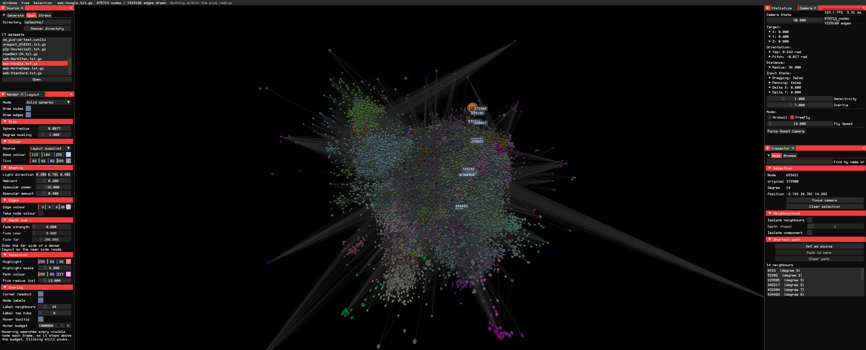
Solid mode solves a ray-sphere intersection per fragment, in view space:
vec3 rayDirection = viewRay();

float b            = dot(rayDirection, center);
float discriminant = b * b - (dot(center, center) - radius * radius);

if (discriminant < 0.0) discard;

float t = b - sqrt(discriminant);
if (t < 0.0) discard;

vec3 hit    = rayDirection * t;
vec3 normal = (hit - center) / radius;
The vertex shader hands down the view-space centre and radius packed into one vec4, the fragment shader rebuilds the ray through its own pixel, and everything visible comes out of those six lines. No sphere geometry, no per-node vertex data beyond the centre.
The comparison I keep coming back to is the Bob-ombs in Super Mario 64. Same trick in spirit, thirty years apart: the thing reads as a smooth round ball and the geometry underneath is emphatically not one. Only the place you cheat moved. The N64 cheated at the vertices, shading a chunky low-poly body as though it were a perfect sphere. Here the cheat is in the fragment, and the shape is not approximated at all, it is solved exactly for every pixel that lands on it.
Two details that are cheap to get right and expensive to get wrong.
The ray reconstruction needs no matrix inverse. The projection is a symmetric perspective, so clip.xy = (proj[0][0] * x, proj[1][1] * y) and w = -z. Dividing the NDC by those two diagonal terms inverts it, and whichever way the projection flips Y rides along in the same uniform.
The depth has to be written. The rasterizer gives every fragment of a point sprite the depth of the sprite's centre, one value across the whole thing, which puts every sphere on a flat card. Writing the depth of the actual hit makes spheres intersect properly and lets the edge pass depth test against a real surface. But writing gl_FragDepth normally kills early-Z, and on a million-node cloud losing depth rejection is fatal. One line fixes it:
layout(depth_less) out float gl_FragDepth;
The hit is on the near side, so it is never further than the centre depth the rasterizer already computed. Declaring that keeps early-Z.
The sprite that clipped its own sphere
The bug that took longest to understand: spheres came out clipped at the edges of their point sprite. The sprite was sized radius / viewDepth, which is the obvious thing and is wrong in two independent ways. The silhouette of a sphere is its tangent cone, wider than the disc through its centre, and perspective stretches that cone further the further off-axis the node sits. Both errors grow toward the corners of the screen, which is where it looked worst.
The exact bound falls out algebraically. Project the sphere onto the plane spanned by the view axis and one screen axis and you get a circle of the same radius, so the extreme of over the sphere is the tangent from the eye to that circle:
with the angle of the centre off axis and the tangent half-angle. Expand the cosines in terms of , and and the trigonometry cancels:
Both axes get evaluated and the wider wins, because a point sprite is square and the projection is not once the viewport is not. A non-positive denominator means the eye is inside the sphere, and the size is pinned to the viewport so the surface stays covered instead of being clipped away. gl_PointSize is clamped to the device's pointSizeRange[1], since writing past it is undefined.
Additive splats
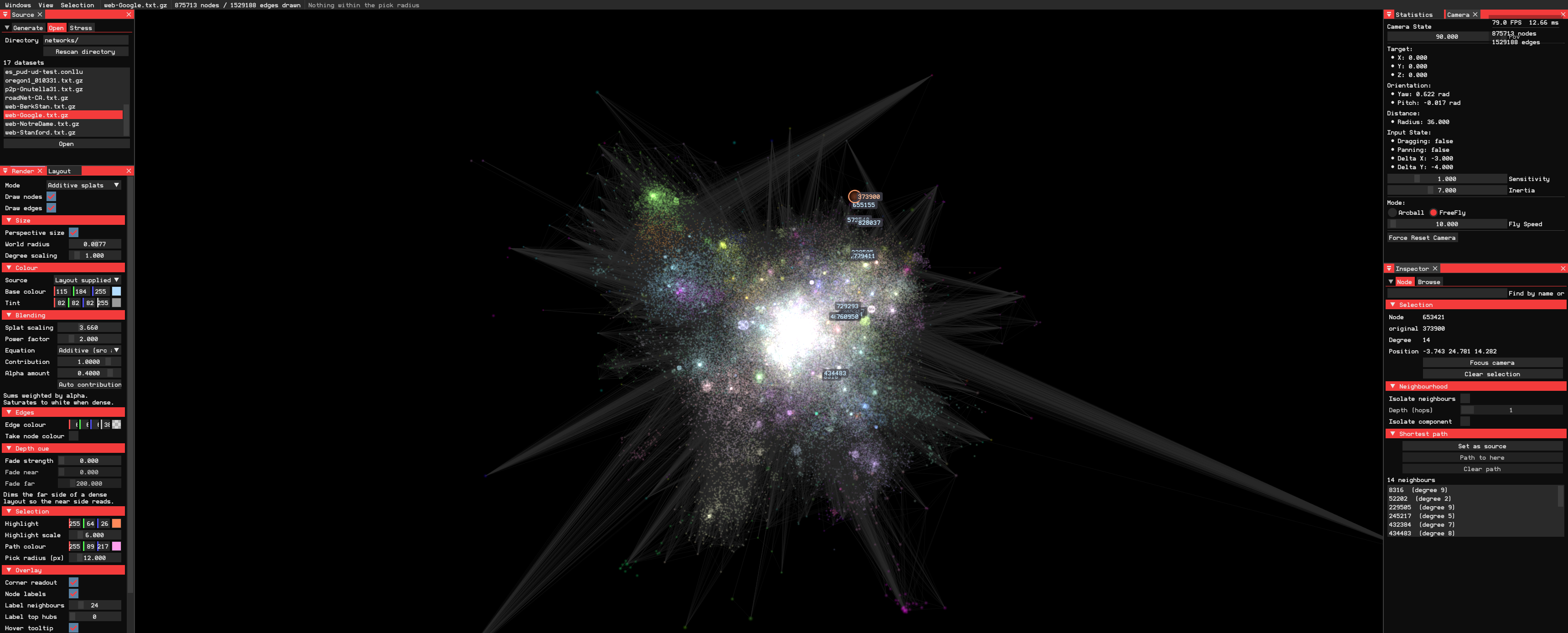
The second mode drops all of it. No intersection, no normal, no depth write, no lighting:
vec2  offset  = gl_PointCoord.xy - vec2(0.5);
float falloff = exp(-pow(length(offset * ubo.splatScaling), ubo.powerFactor));

vec3  color = base * falloff * ubo.contribution;
float alpha = falloff * ubo.alphaAmount;
The same blend the GPU particle system uses, for the same reason: density reads as brightness.
Contribution and alpha are separate controls on purpose. Contribution scales the colour, so it governs how much a node reaches the frame under every blend equation; alpha only reaches the frame in the modes whose source factor reads it. There is an auto-contribution button that scales by .
Brightness is a measurement
Because the sum is linear, the brightness of a region is a density readout, not a stylistic glow. Twice as bright is twice as many nodes on that line of sight.
In a Treecapitator layout that means something specific. The layout puts a node near the hub it belongs to, so nodes that are spatially close are nodes that share connectivity. A bright patch is a region of tightly connected nodes packed together, and you read the strength of a community straight off the image without computing anything. The gradient around it tells you how fast that density falls off.
Solid mode cannot do this. An opaque surface saturates at one node: fifty behind it look like one.
Edges in the node's colour
Edges default to a flat dim grey so they read as structure without competing with the nodes. Turning on "take node colour" makes each edge inherit its node's colour, and since Treecapitator already colours a node by blending in its hub's colour, every hub ends up owning a visibly coloured fan of edges.
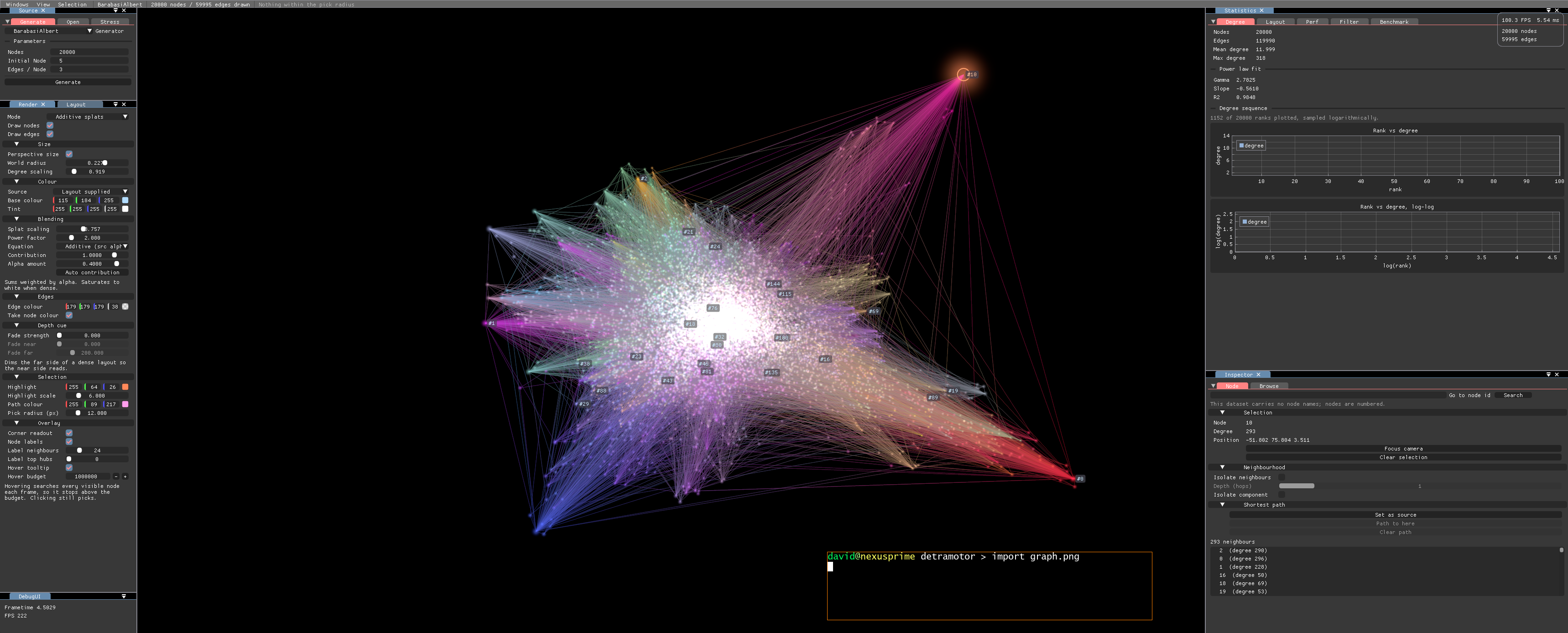
That is a generated Barabási–Albert graph rather than a loaded one: 20,000 nodes, 3 edges per new node, straight out of the Generate tab. At that size everything is comfortable (180.3 FPS, 5.54 ms), which makes it a good picture for looking at rather than for benchmarking.
Both effects show up at once. The core is white because that is where the density is, and each big hub has coloured its own tree of edges, so spokes that would be an undifferentiated grey haze separate into distinguishable communities. The magenta fan going up to the right and the red one going down to the right are two different hubs, visible without clicking anything.
One vertex stream, several jobs
At ten million nodes every interpolant the vertex stage exports is paid ten million times a frame, so a few things ride along in odd places:
- The colour attribute is
R8G8B8A8_UINT, notUNORM, and travels to the fragment shader as the packeduintit already was. Sphere mode went from 8 exported floats to 5, additive from 4 to 1. - The alpha channel of that colour carries the normalised degree, so point size can follow connectivity without a second vertex stream.
- Selection is resolved in the vertex shader against
gl_VertexIndex, so highlighting costs nothing per frame and needs no second draw. - The projection is applied by hand from its five non-zero entries instead of as a second full
mat4multiply.
The last two measured neutral: 167.4 FPS against 169.8 before, inside run-to-run noise. They stayed because they are strictly less work, not because they bought anything.
The numbers
First, a confession: every FPS number this thing produced for its entire life was a vsync floor. The swapchain was hardcoded to FIFO, so every measurement reported the display refresh rate and nothing about the renderer. There is now an environment variable for the present mode, and immediate is where the real numbers live.
RX 7700 XT, 10 million node synthetic point cloud, 4 second runs, first 30 frames discarded so pipeline compilation and first-touch page faults stay out of the sample:
| run | avg | median | 1% low | Mpoints/s |
|---|---|---|---|---|
| solid (ray-traced spheres) | 5.98 ms, 167.4 FPS | 166.8 | 156.0 | 1674 |
| additive (blended splats) | 5.35 ms, 187.0 FPS | 186.5 | 177.9 | 1870 |
| idle, nothing drawn | 0.54 ms, 1845 FPS | 1906 | 1287 | n/a |
At 2 million nodes: solid 755.8 FPS, additive 813.1 FPS, idle 1860 FPS.
Additive is faster here, while in the Google graph screenshots solid runs at 169.9 FPS and additive at 79.0. Both are true. In the benchmark the camera frames the whole cloud, nodes project to about one pixel, nothing is fill bound, and the 0.63 ms solid gives up is the depth buffer plus the per-fragment depth export. In the screenshots the camera is close enough that splats cover real screen area, nothing is discarded or depth rejected, so additive pays full fill rate over every quad.
Which mode is faster depends entirely on where the camera is.
Where the frame time goes
Both modes land at 1.87 to 2.08 Gprim/s. That number being the same in both is the tell: the limit is the geometry front end, one primitive per node.
- Not ALU. Roughly 9000 ops of headroom per vertex at this rate.
- Not bandwidth. 160 MB/frame of vertex fetch is 29 GB/s out of 432 available.
- Not fragments, at that framing.
Getting past ~1.9 Gprim/s means not emitting a primitive per node at all: a compute shader splat with 64-bit depth atomics, which the device supports. That is a real rewrite and I have not started it.
Three things burning CPU
Idle costs 0.54 ms a frame now, which is how I know the rest is GPU draw. Getting there meant finding three things doing per-frame work that only changed when something changed.
- The statistics panel handed the plotting library the entire degree sequence every frame. Ten million points, two plots. Now decimated once at load to at most 2048 logarithmically spaced ranks (log spacing, because uniform sampling of a heavy tail gives you two thousand copies of degree 1 and misses every hub). The power-law fit still runs over the full sequence, only the plot is sampled.
- The Open panel ran the directory scan, one syscall per entry, on every frame it was visible. Now cached behind a Rescan button.
- Every buffer upload allocated a fresh staging
VkBufferof the full size. A 160 MB allocate and free per frame while streaming. Now a two-deep per-graph ring: the engine keeps two frames in flight, so by the time the ring comes back around, the frame that read that buffer has retired.
Around the renderer
Loading. Edge lists accept space, tab, comma and semicolon separators, skip comments and self-loops, ignore a third column. Node identifiers no longer have to be dense, zero-based or numeric: they get relabelled into a dense range with the original kept as a name. Previously a sparse id space sized the graph to the largest number in the file. A .labels sidecar can replace those names. The whole load runs on a worker thread.
The scene layer sits between the graph and the buffers: a filter chain (component isolation, neighbourhood isolation, minimum degree, node budget), colour modes (degree, uniform, hops from selection, component, position, layout), and analyses computed on demand and cached until the graph changes. Selection and current path are pinned so a filter never removes what you were looking at. Nothing in there runs per frame unless something changed.
Picking is a parallel screen-space nearest search over the visible buffer. O(V), a few milliseconds at ten million nodes, which is fine for a click and hopeless for a frame. So hover picking stops above a budget (a million nodes by default) while clicking still picks, because a click pays for its own search.
The panels were the other surprise. ImGui writes a widget's label after the widget and gives the widget 65% of the window width, so in a docked panel the names run off the right edge and the only way to read them is to drag the panel wider. Every control now goes through a two-column table helper, names left and controls right, with the name column sized to fit its content. That helper got promoted into the engine, since the problem is not specific to this application.
Still open
- Quitting aborts. VMA asserts its memory blocks are empty on teardown and something still holds device memory when it goes down. The demo releases its graph and renderer from a new shutdown hook and that is not enough. It predates the port; the clean-close path just made it visible every run.
- The camera controls build the projection with the GL depth range convention while Vulkan uses another, squeezing the scene into about 1% of the depth range. Ordering works, precision is poor. It touches every depth-using component, so it is left alone.
- The force-directed hub optimisation pass in Treecapitator indexes two different arrays in its integration step and its force loop, so it moves the wrong nodes. Left faithful to the original experimental algorithm rather than quietly fixed, since the academic writeup describes what the original did.
The application is not released yet. When it is I will link it here and from the academic page, which still documents the algorithm and the parameter study from the OpenGL version. All of that still applies. The layout did not change, only the thing drawing it.