Detravisualizer
A 3D graph layout and visualization tool for large power-law networks, built in C++ with OpenGL. The core contribution is Treecapitator: a degree-based layout algorithm designed specifically for graphs that exhibit small-world characteristics and a power-law degree sequence.
Results
The following renders show Treecapitator running on networks at different scales. Colors encode community structure via degree-propagated HSV assignment; alpha blending exposes connection density even in graphs with tens of millions of edges.
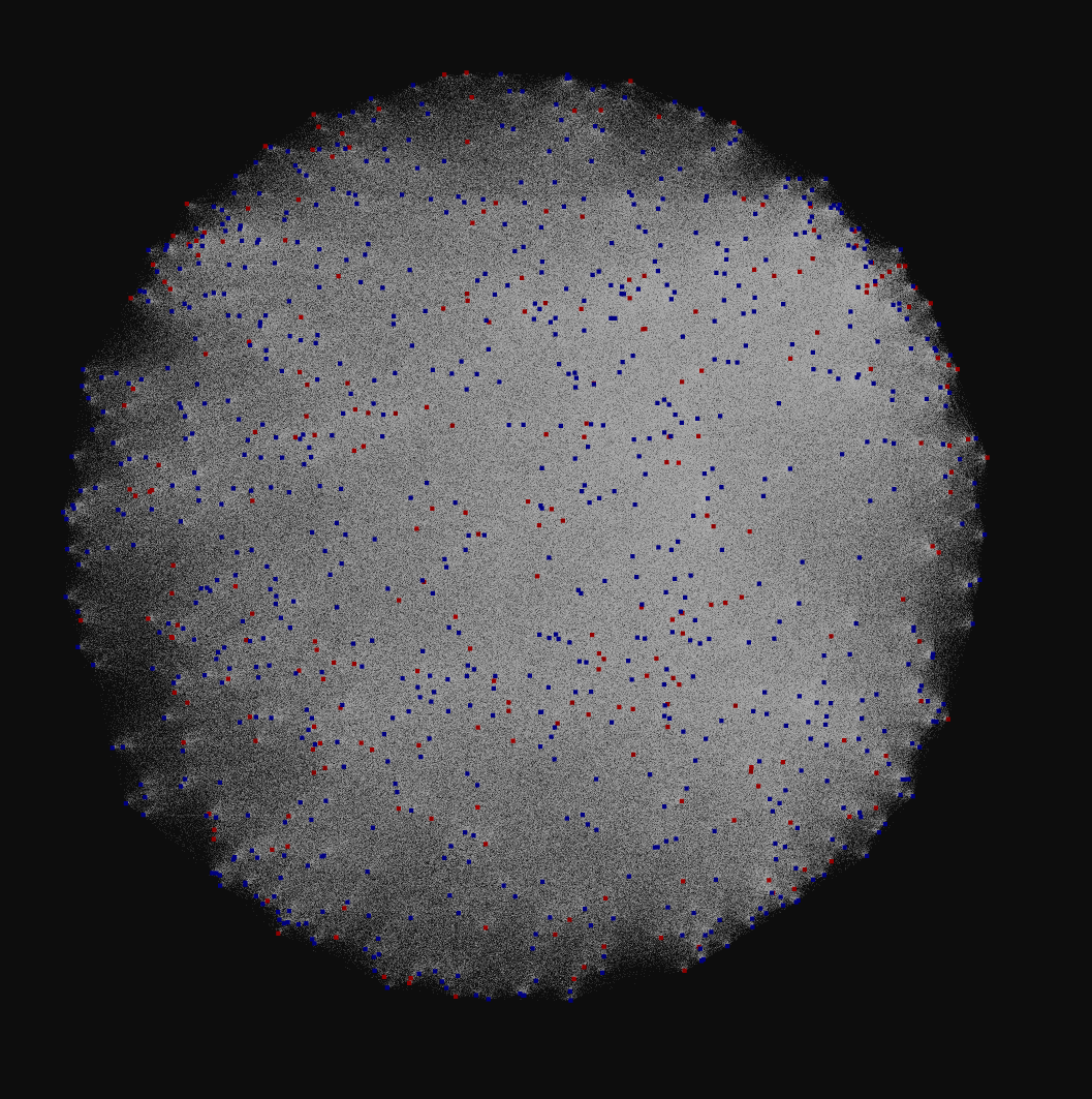
Barabási–Albert, 10 million nodes — structured hubs emerge clearly:
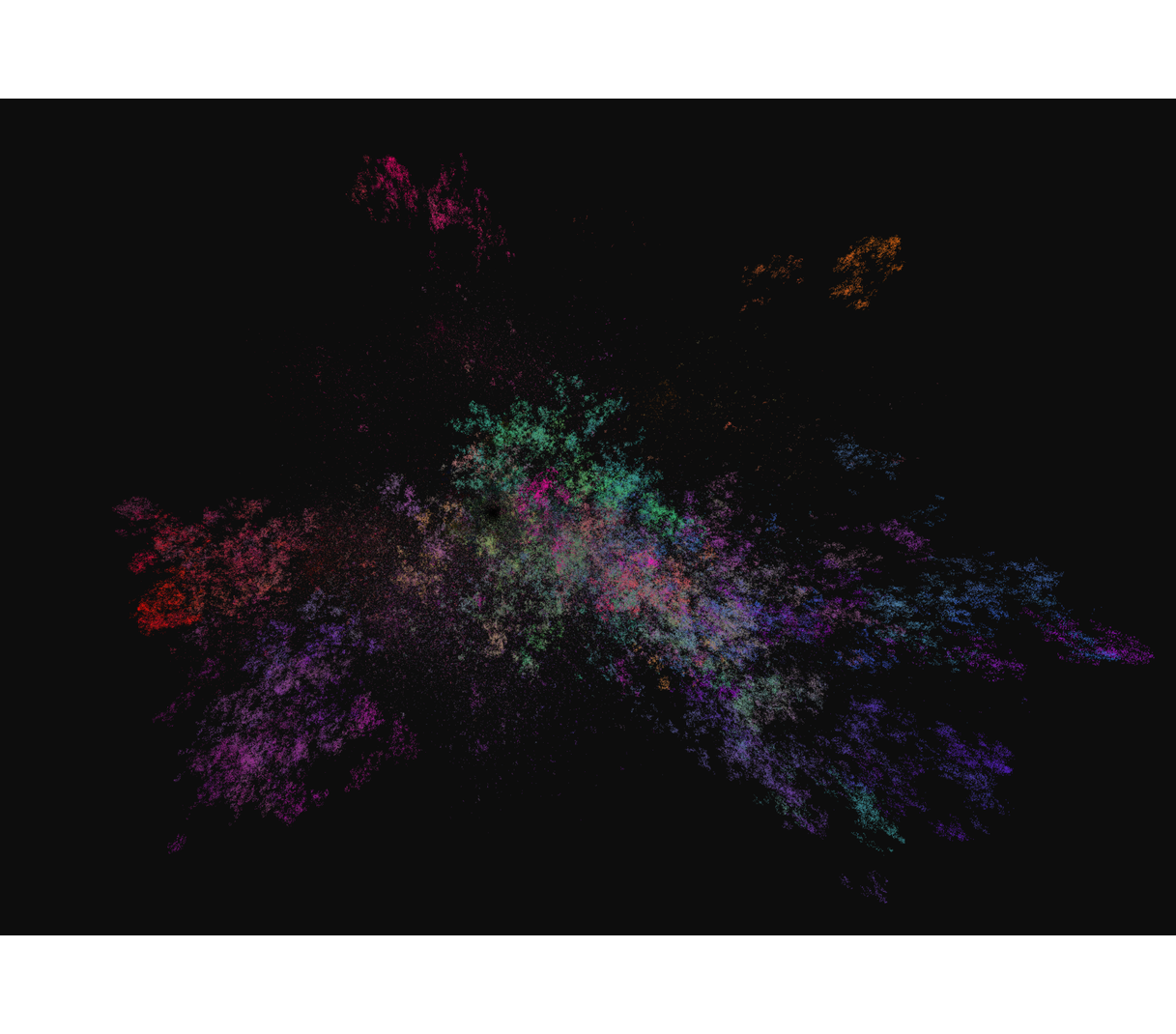
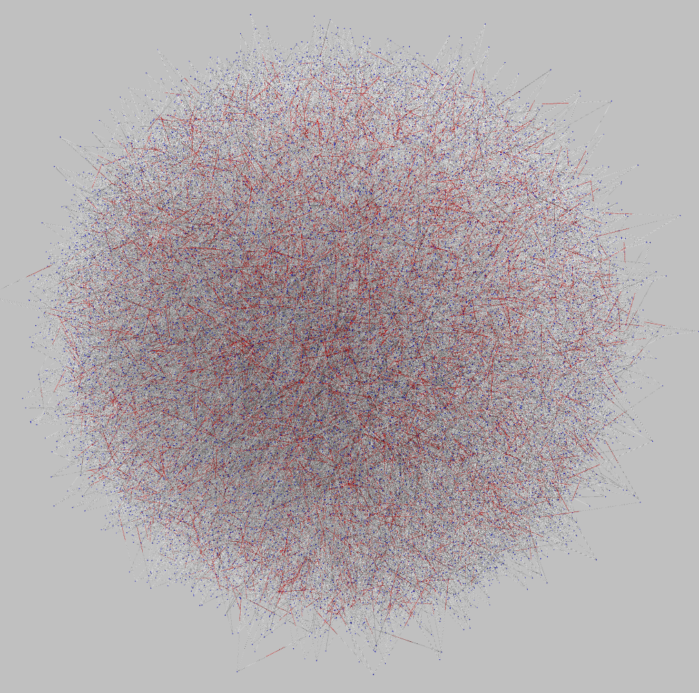
Left: Treecapitator on 10M node BA network (b=120, c=0). Right: Graphia on 1M node BA network. The stock algorithm collapses all nodes into an undifferentiated mass.
Factor Graph, 150,000 nodes — deterministic and randomized variants:
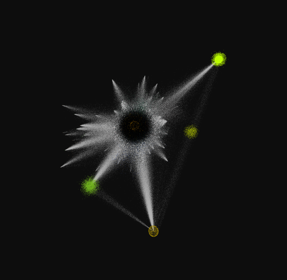
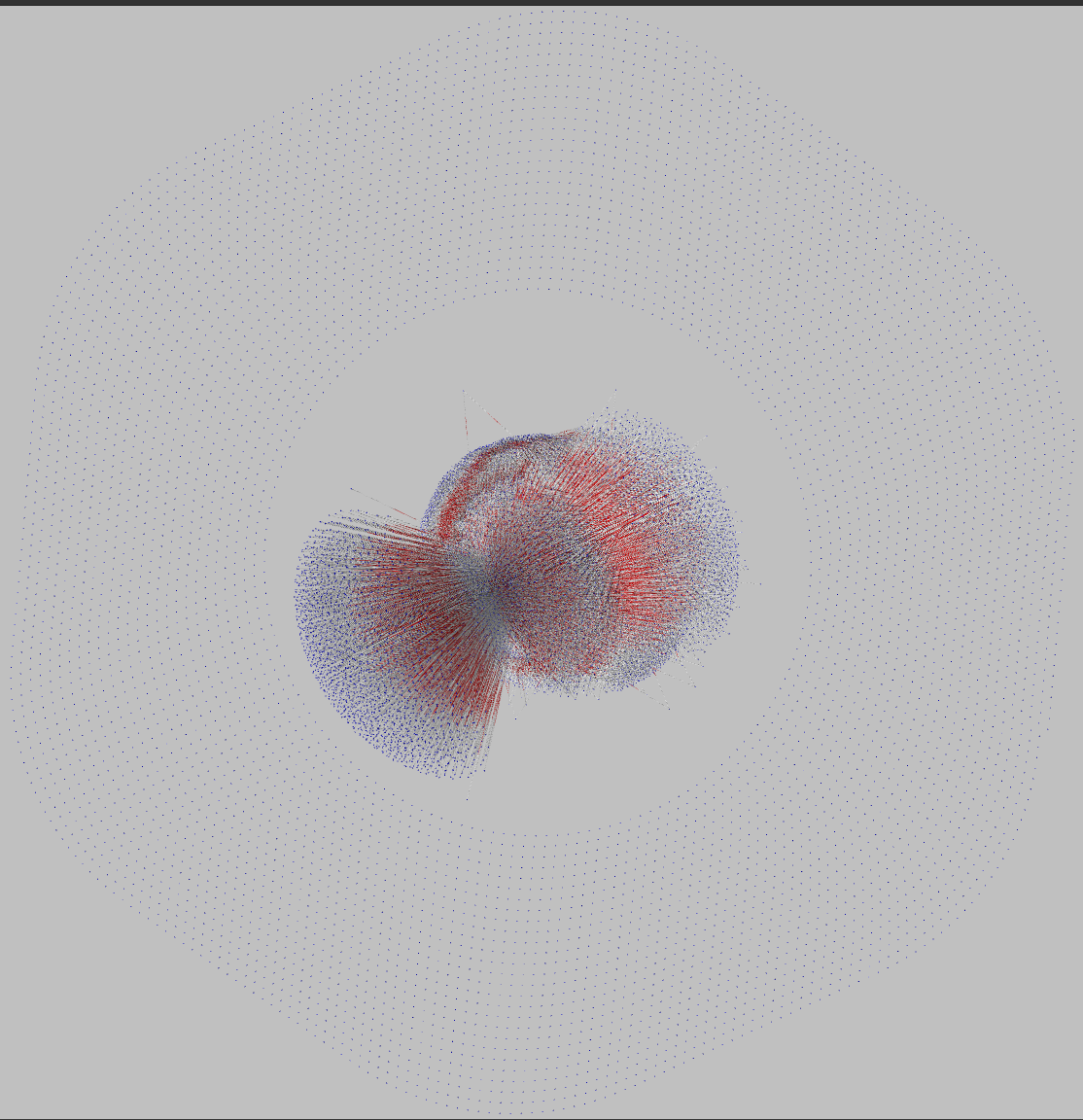
Left: Treecapitator on the Factor Graph model (150k nodes). The divisibility-based structure creates characteristic bubble clusters. Right: Graphia collapses the same network into a featureless ball.
Rendering parameters — alpha and perspective:
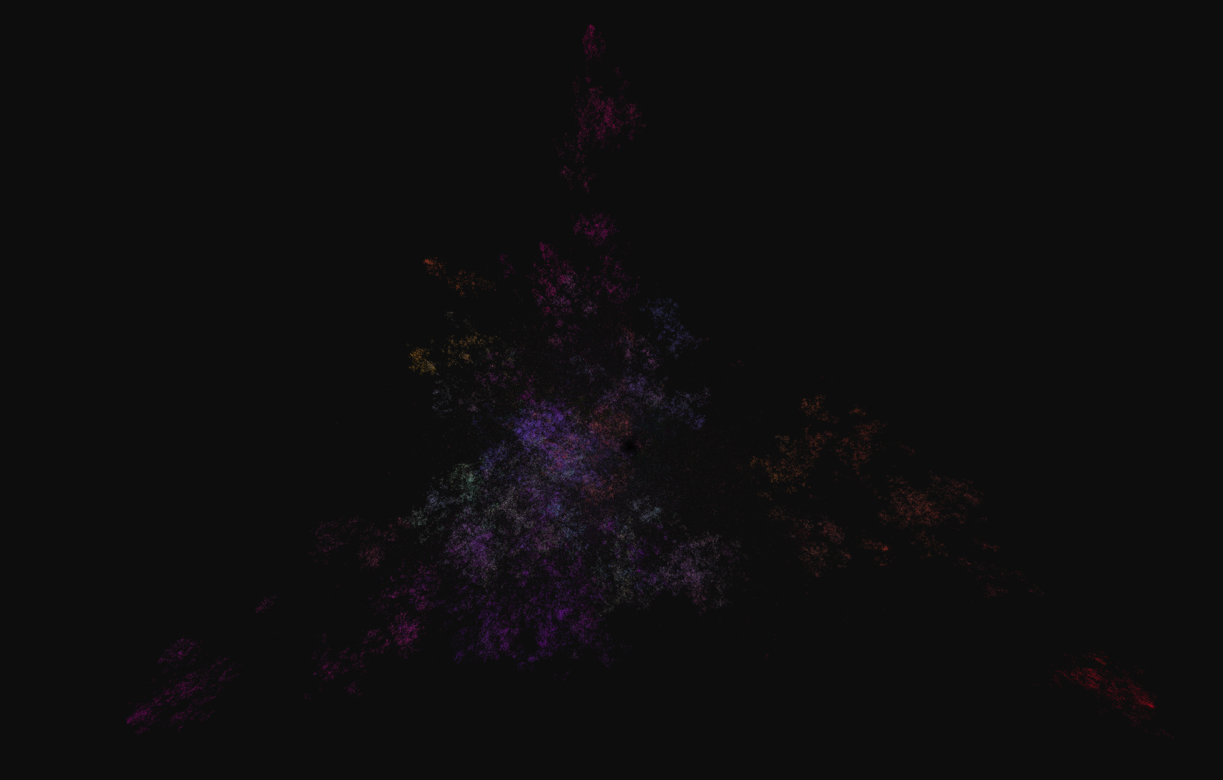
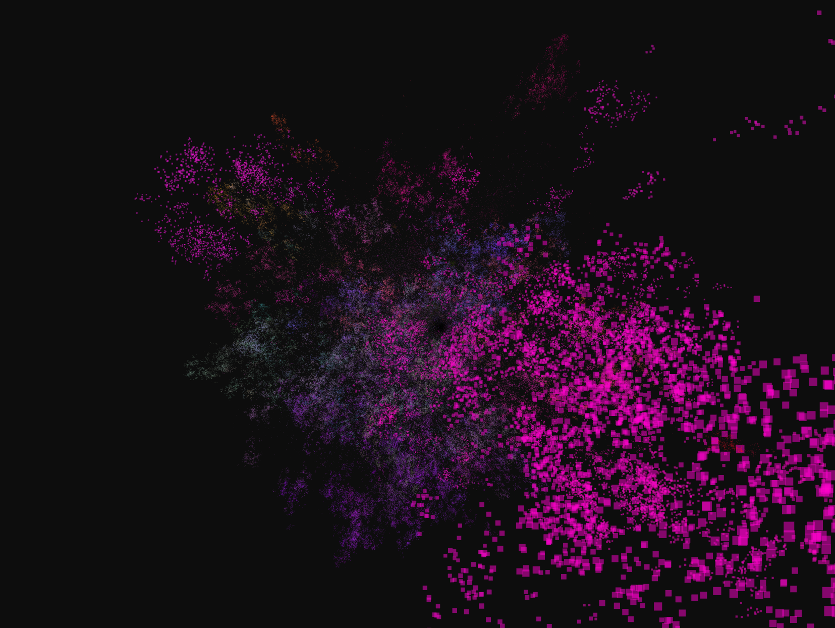
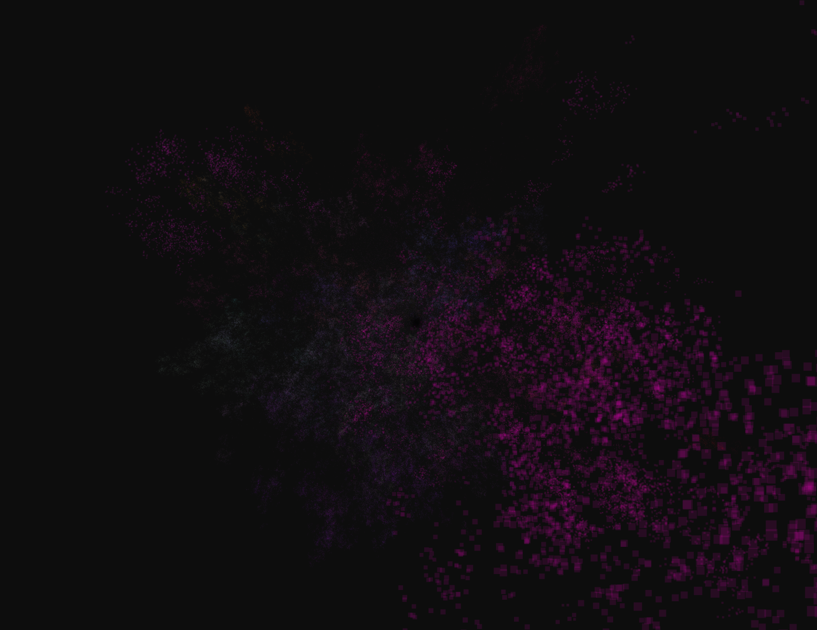
Effect of alpha transparency on a dense Barabási–Albert network. Low alpha reveals internal structure that full-opacity rendering hides entirely.
Demo
The Problem with Power-Law Graphs
Real-world networks — social graphs, web link graphs, citation networks, linguistic dependency trees — consistently exhibit a power-law degree distribution: a small number of nodes have very high degree (hubs) while most nodes have very few connections. Formally, for a graph , the degree distribution follows:
for some exponent .
Standard layout algorithms (force-directed, spring-embedded, Fruchterman–Reingold) treat all nodes equally. Applied to a power-law graph, the high-degree hubs exert enormous attractive forces on their neighbors, pulling the entire network toward the center. The result is an impenetrable central mass with no readable structure.
The five research questions this work set out to answer are:
| Question | |
|---|---|
| RQ1 | Does the presented layout offer a visually clear representation for power-law degree graphs? |
| RQ2 | Is the representation useful? |
| RQ3 | What is the behaviour with other graph types that do not follow a power-law degree sequence? |
| RQ4 | Does the layout offer a representation improvement over natural graphs? |
| RQ5 | How do the parameters change the behaviour? Are they equally relevant? Are they graph-dependent? Can they be fine-tuned? |
A New Power-Law Model — Factor Graph
To test the layout at scale, a new synthetic power-law graph generator was built alongside the visualizer. I call it the Factor Graph model.
Traditional power-law models (Barabási–Albert, preferential attachment) simulate network growth step by step: each new node is connected to existing nodes with probability proportional to their degree. This makes large-scale generation expensive.
The Factor Graph instead evaluates edge connectivity between any two nodes in using a closed-form divisibility rule.
Definition
We first define a labelling function that maps each vertex to a natural number from a continuous range over :
Each node is associated with a consecutive label starting from 2. The edge set is then defined by a divisibility connectivity rule:
where is a constant controlling the power-law exponent. This rule connects a pair if and only if either divides or divides in this -weighted sense.
Randomization
To remove the deterministic structure introduced by integer labeling, a hashing function (random bijective mapping) can be applied:
This randomizes the endpoints while preserving the small-world statistical properties.
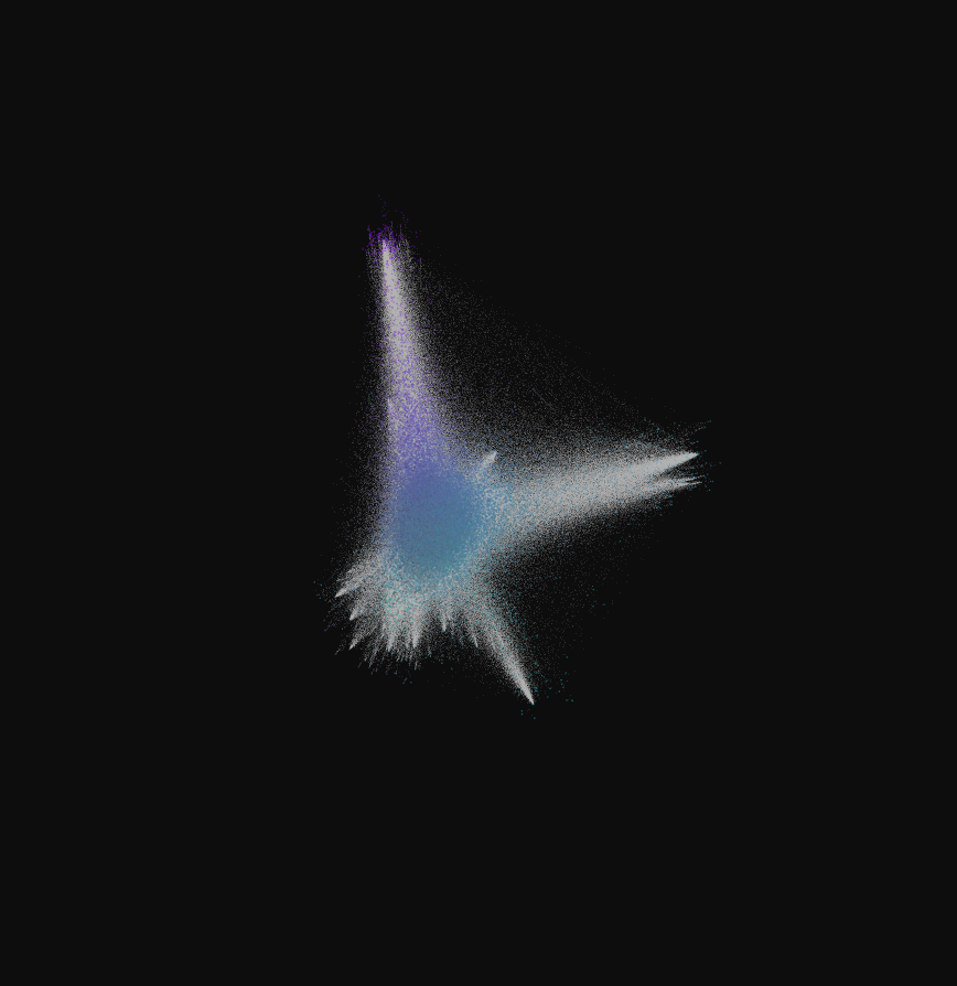
Left: deterministic Factor Graph (150k nodes) — the divisibility structure is directly visible as discrete bubble clusters. Right: randomized Factor Graph (50k nodes) — the clustering dissolves under the hash permutation while the heavy-tail degree distribution is preserved.
Statistical Analysis
For a node with label , define the right-neighbor set as all nodes such that divides :
The expected size of is the number of values whose -power does not exceed :
For the left-neighbor set , the probability that divides a uniformly random label is:
Therefore the expected size of converges when :
The average degree of a vertex then satisfies:
This establishes the heavy-tail behaviour characteristic of power-law graphs. The model follows a strict power-law distribution until a breaking point beyond which the tail decreases at a lower rate than expected — a 2-regime function that distinguishes it from standard preferential attachment.
Treecapitator — The Layout Algorithm
The algorithm sorts all nodes in descending degree order and processes each node heuristically, looking only at the node's degree and its immediate connections. For each node , it computes three position vectors , , and , then blends them into a final 3D position.
Notation
Let denote the degree of node , and its 3D position. For a node set with fixed ordering, define:
For each node we also need — the set of neighbors with strictly higher degree than :
Component A(u) — Attraction to Higher-Degree Neighbors
places a node close to its highest-degree neighbor. The softmin function provides a differentiable approximation to argmin, controlled by temperature :
Then:
The rationale is that a low-degree node is unlikely to find a structurally significant connection outside its local hub. Placing it close to the minimum-degree member of (its most local hub) preserves local topology while allowing hubs to determine the global structure.
Component B(u) — Degree-Proportional Scatter
spreads nodes away from the origin in a random direction, scaled by parameter :
For high-degree nodes, dominates the final position. This is the mechanism that pushes hubs outward — in direct contrast to force-directed methods that pull hubs toward the center.
Component C(u) — Anti-Determinism Jitter
adds a small random displacement to prevent degenerate configurations where many nodes share identical adjacency lists and would otherwise collapse to the same position:
From the definition .
Position Blending
The final 3D position for node is a linear interpolation over the normalized degree :
For the highest-degree nodes (), the position is dominated by : they are placed far from the origin in a random direction. For the lowest-degree nodes (), the position is dominated by : they cluster around their local hubs. The result is a natural hierarchical separation where hub degree directly corresponds to spatial isolation.
Optimization Pass
High-degree hubs placed by may end up spatially close to unrelated hubs purely by chance. An optional force-directed optimization corrects this for the top- fraction of degree holders. Select the hub set:
Then apply Euler integration of repulsive forces between all pairs in :
where constrains each hub to its initial sphere, preventing scale collapse. Iteration continues until convergence:
Node Colouring
The colour of a node follows the same positional logic. Define and as analogues to and but in HSV colour space (random Hue, fixed Saturation and Value = 1) rather than 3D position space. The final colour:
where . High-degree nodes receive a unique random colour; low-degree nodes inherit a blend of their hub's colour. This allows color to serve as a visual proxy for community membership — nodes connected to the same hub cluster in both space and colour.
Tunable parameters summary:
| Parameter | Role |
|---|---|
| Controls overall scale of the network; dominates position of hubs () | |
| Controls jitter magnitude for low-degree nodes (); prevents degenerate overlaps | |
| Controls greediness of ; selects strictly the minimum-degree neighbor |
Results — Synthetic Networks
Networks were generated with the following default parameters unless otherwise noted: , , .
Barabási–Albert vs. Erdős–Rényi
The most revealing comparison is between BA and ER models. BA exhibits preferential attachment (power-law), while ER has a binomial degree distribution.
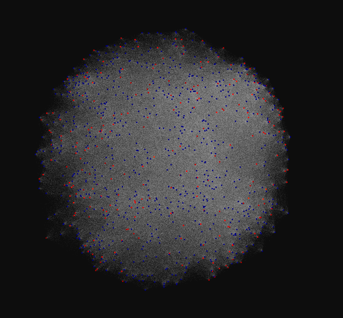
Left: BA model (Treecapitator) — hubs disperse, color communities clearly visible. Right: ER model (p=0.5, Treecapitator) — nodes distribute uniformly on a sphere surface with no structure, correctly reflecting the absence of power-law degree distribution.
This contrast validates the algorithm's design: when there are no hubs ( has no preferred direction), dominates and all nodes scatter uniformly on a sphere.
Erdős–Rényi — Varying Connectivity Probability
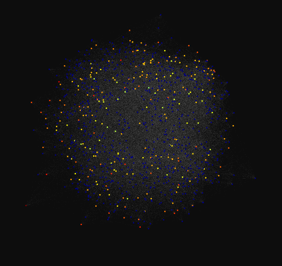
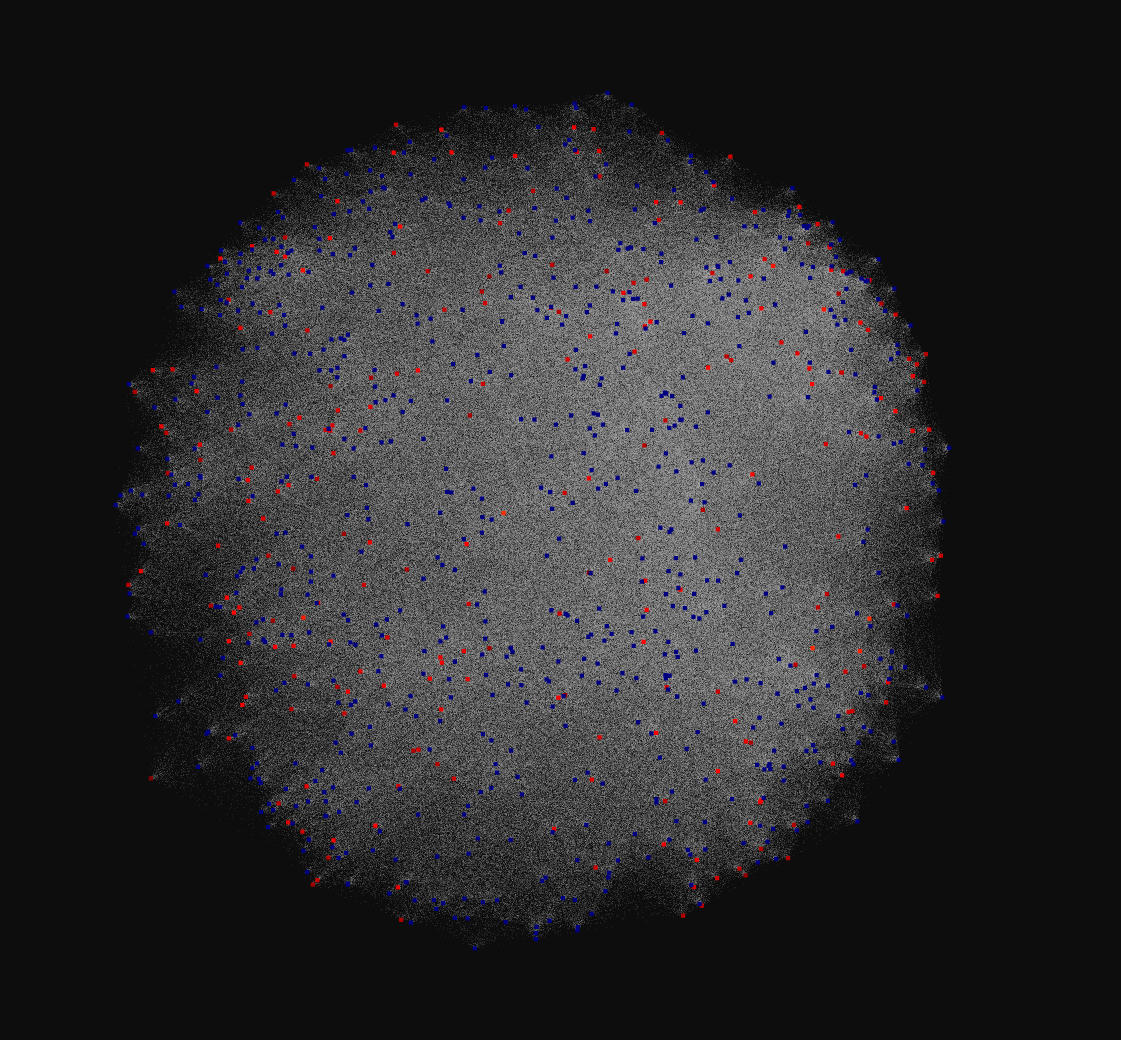
Erdős–Rényi with N=1000 nodes and p ∈ {0.088, 0.5, 0.957}. As p increases (every node approaches the same high degree), the sphere fills in from the inside. Decreasing p scatters sparse nodes outward from an empty center.
Watts–Strogatz — Varying Rewiring Probability β
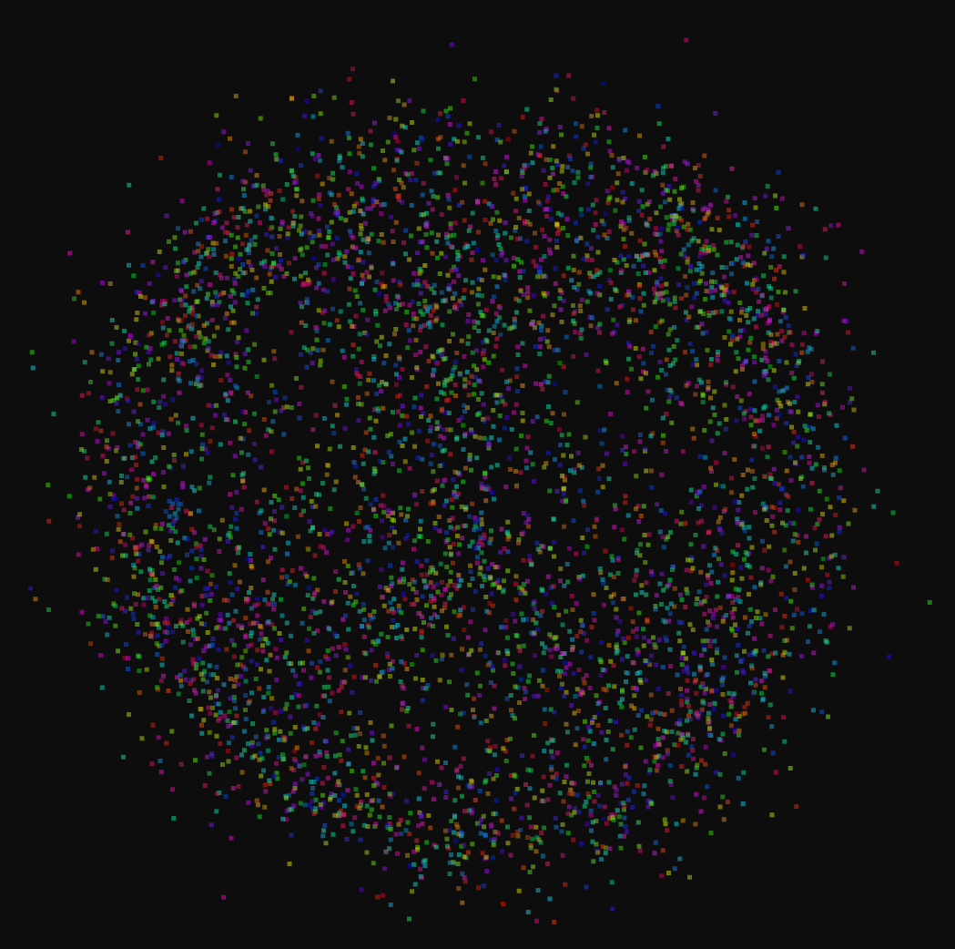
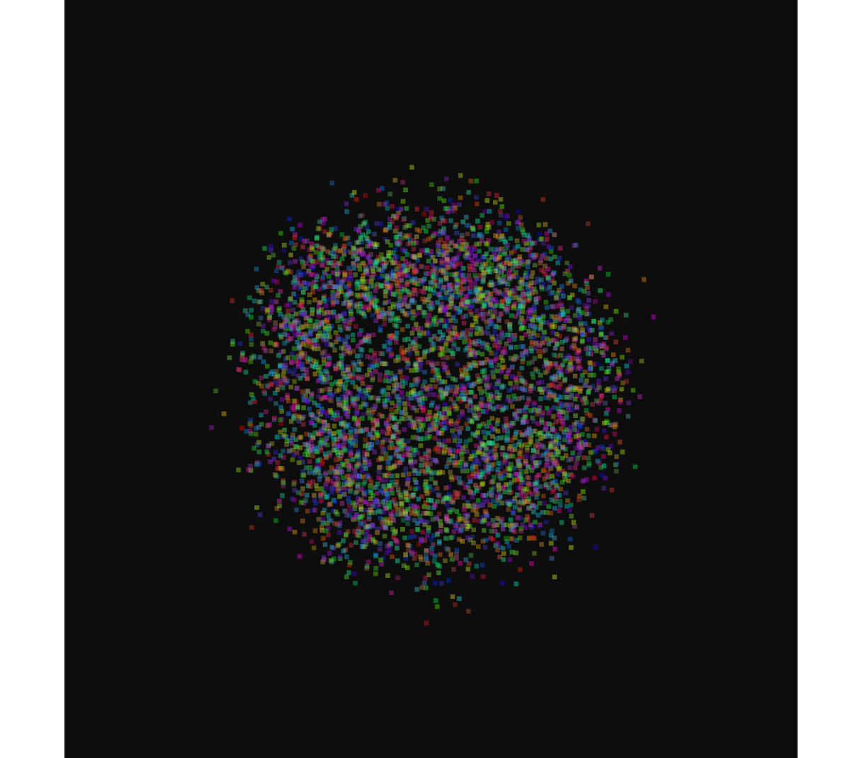
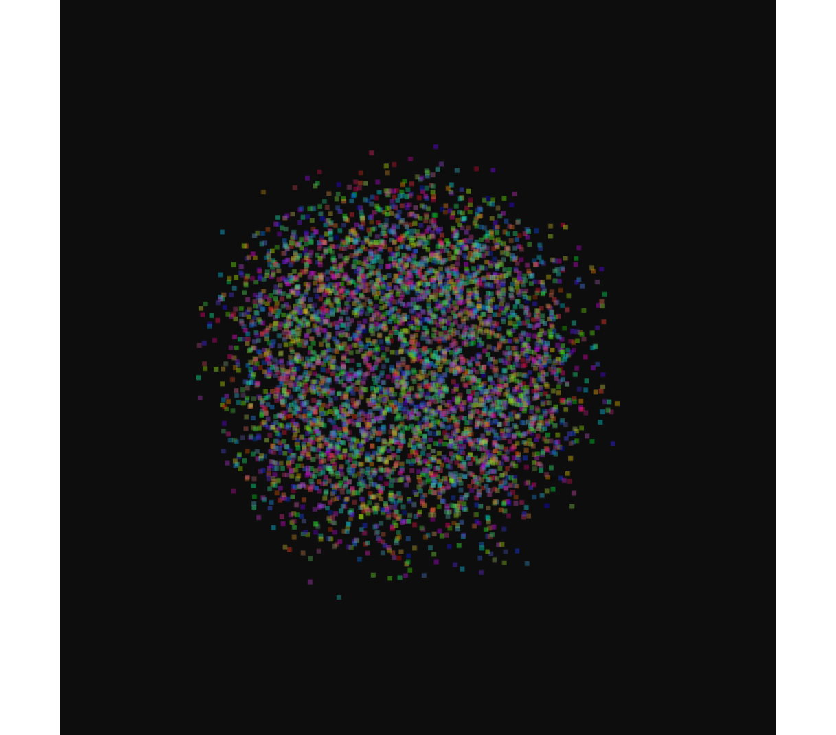
Watts–Strogatz (N=5000, k=4) with β ∈ {0, 0.1, 1}. At β=0 all nodes share degree 4 and B(u) dominates every position, producing a perfect sphere. As β → 1 (full rewiring toward BA-like structure) internal organization appears.
A key theoretical consequence: in a regular graph where all nodes have the same degree, for every node, meaning everywhere. The result is a sphere of radius with jitter — which is exactly what the β=0 result shows.
Barabási–Albert — Varying γ Exponent
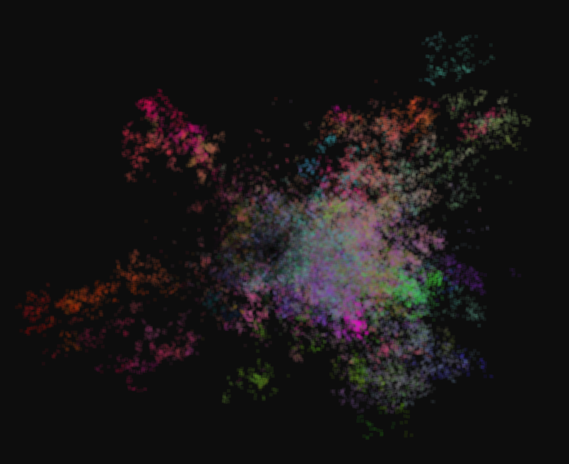
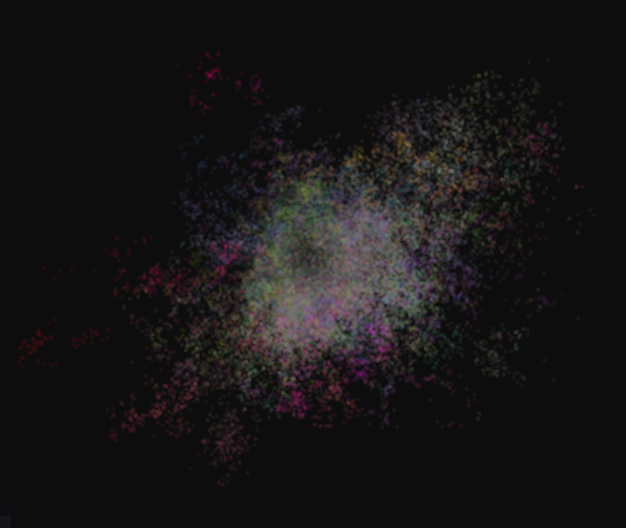
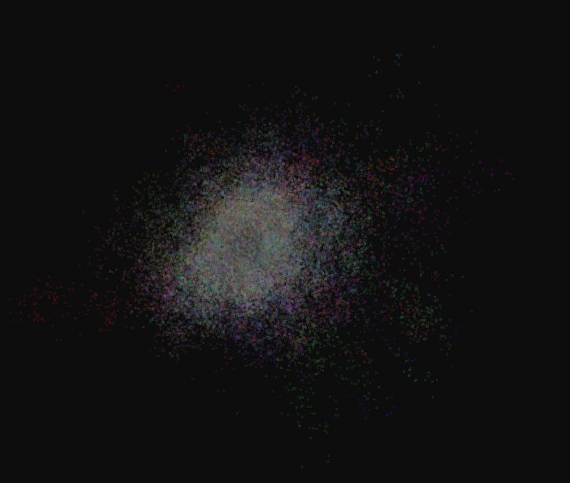
γ ∈ {2.82, 2.83, 2.86}. Even a marginal increase in the power-law exponent produces a rapid fall in perceived structure. As γ increases, the degree distribution becomes more uniform and the layout loses its hub-and-spoke character.
Watts–Strogatz vs. Graphia
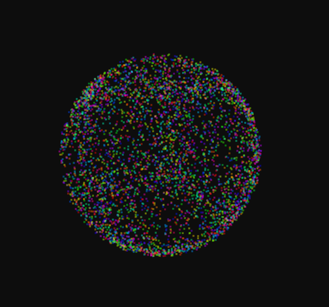
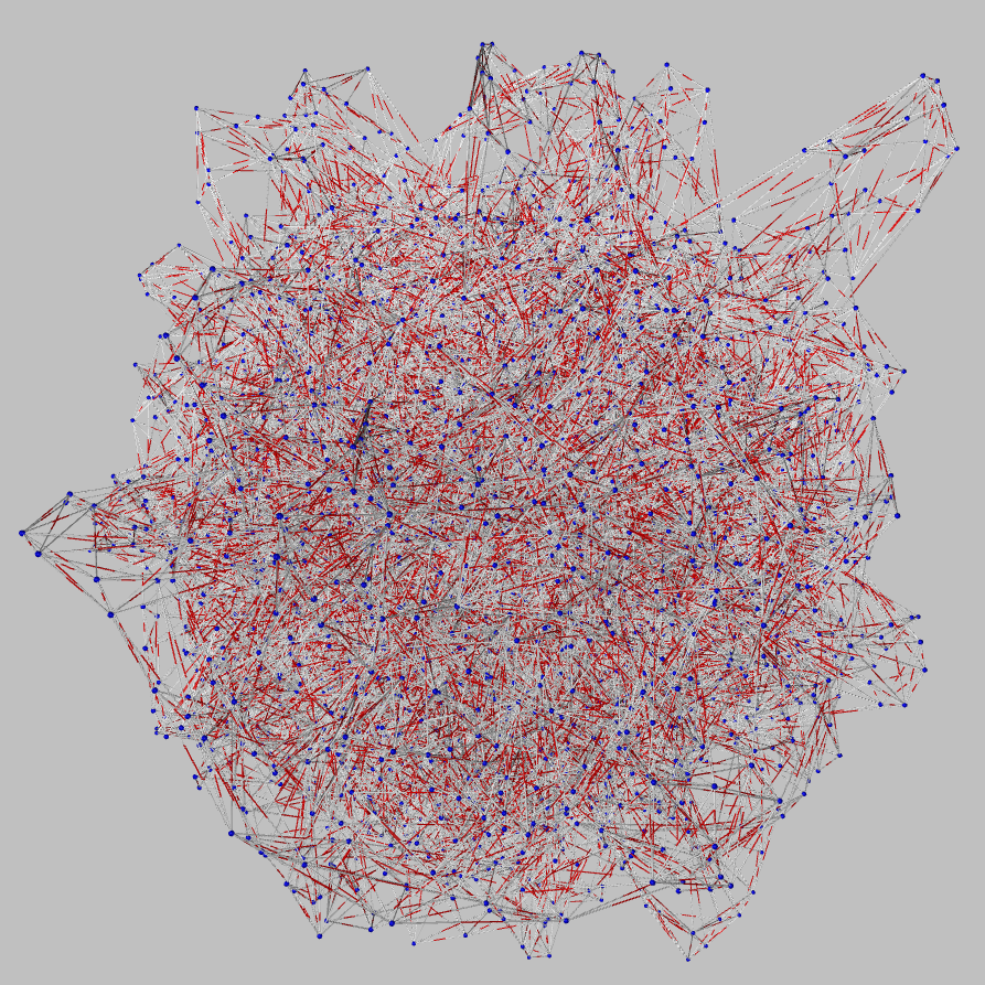
Watts–Strogatz (N=5000). Treecapitator produces a compact sphere at β≈0, reflecting the near-uniform degree distribution. Graphia applies a force-directed approach and produces a ring — structurally different but arguably more informative for this specific model.
Results — Natural Networks
Four real-world networks from the Stanford SNAP dataset were tested.
| Network | N | E | ⟨k⟩ |
|---|---|---|---|
| Email-EU (dir.) | 265k | 420k | 1.58 |
| Google-WebGraph (dir.) | 876k | 5.1M | 5.83 |
| RoadNet-CA (undir.) | 2.0M | 2.8M | 2.82 |
| Catalan Ling. (undir.) | 7.2k | 57.7k | 15.91 |
Email Network (email-EuAll)
A directed communication graph from a large European research institution (Oct 2003 – May 2005). Each node is an email address; an edge from to means sent at least one message to .
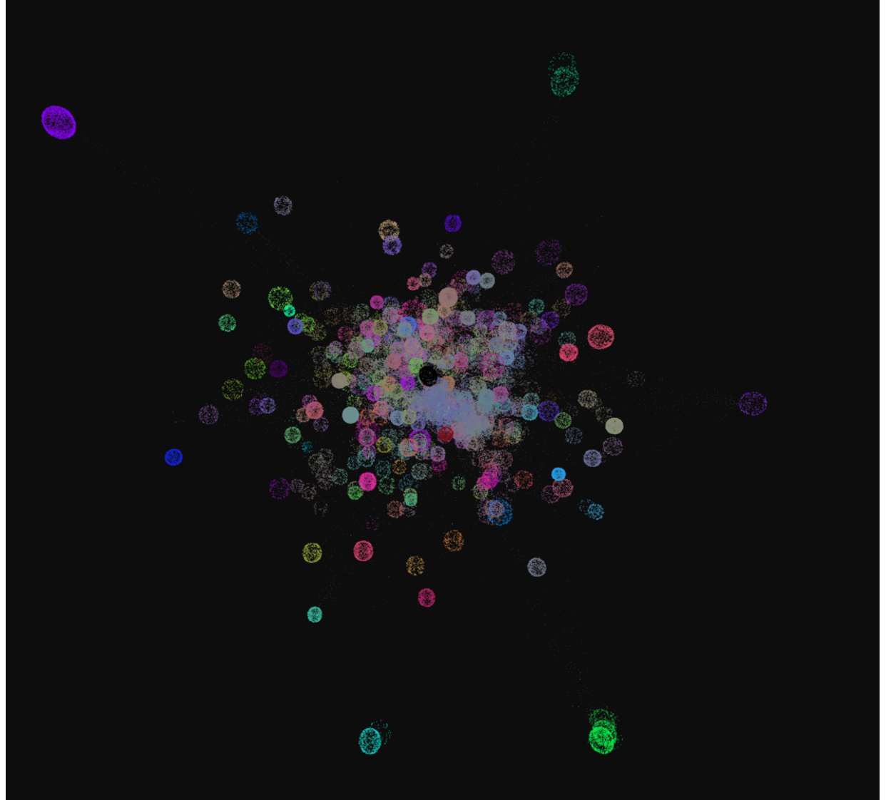
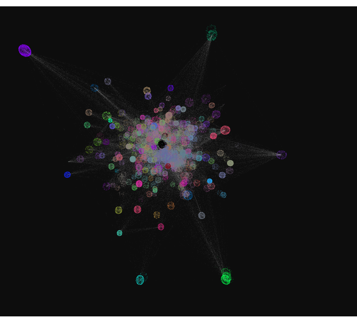
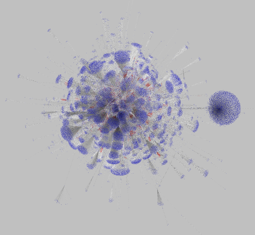
Left and center: Treecapitator (nodes only / with edges). Right: Graphia. Treecapitator detects high-degree hubs and organizes smaller email clusters (bubbles) around them. Graphia produces a more compact but less interpretable layout.
Road Network (roadNet-CA)
California road network: intersections are nodes, road segments are undirected edges.
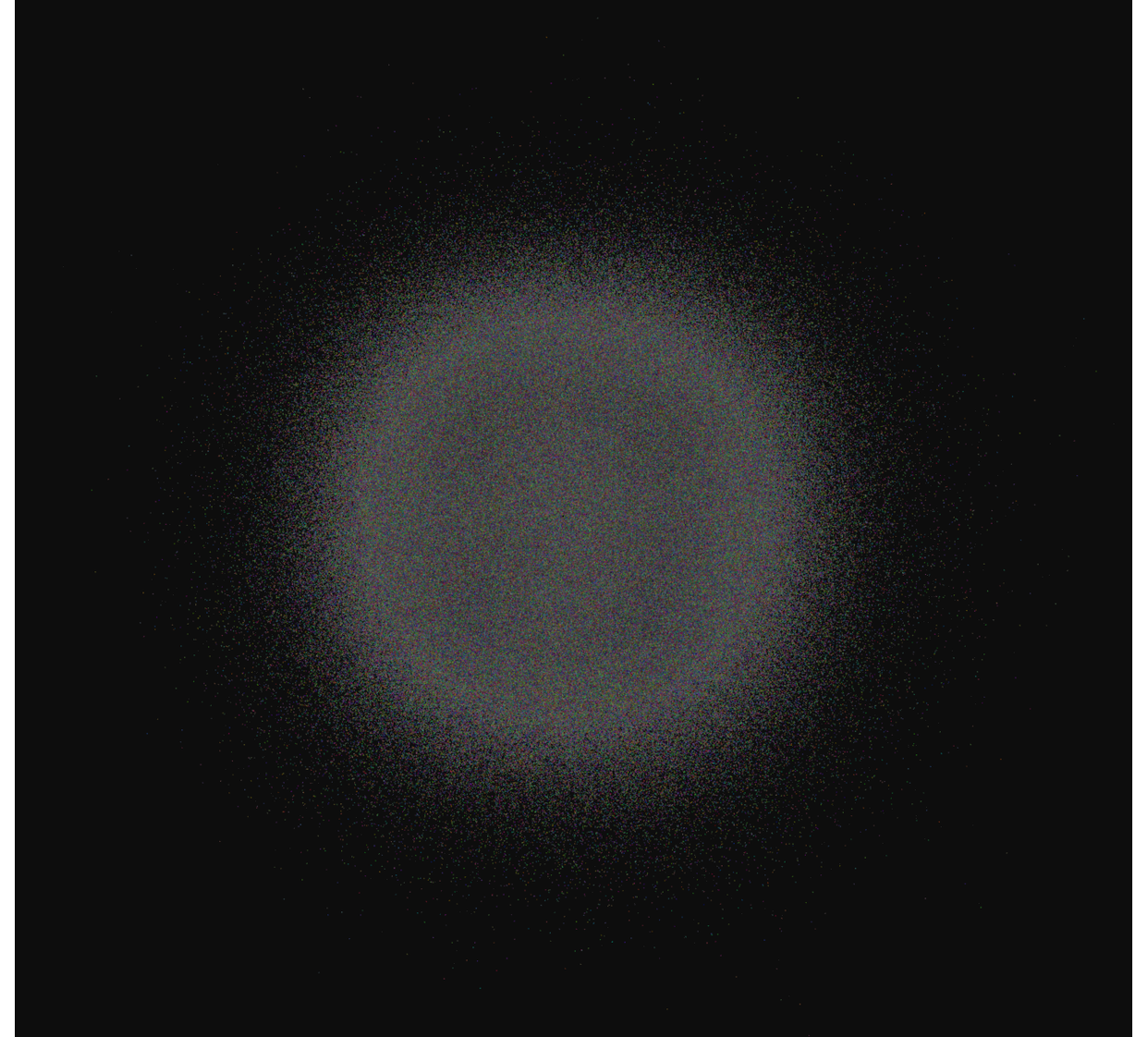
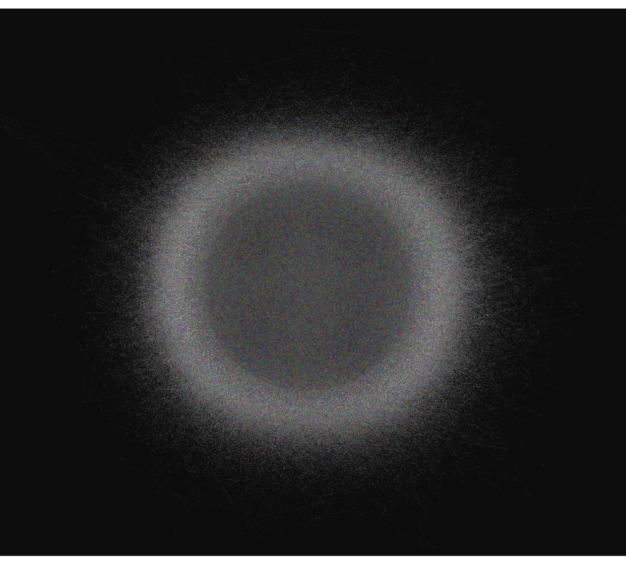
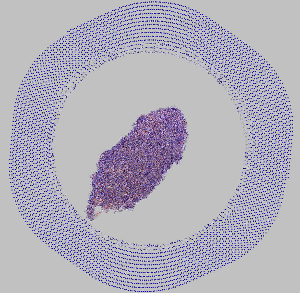
Road networks have a near-uniform degree distribution (most intersections connect to exactly 2–4 roads). Treecapitator correctly identifies this and produces a sphere with no internal structure — visually uninterpretable but statistically honest. Graphia produces a geographically-shaped blob that captures spatial topology better.
Google WebGraph
876k web pages, 5.1M directed hyperlinks.
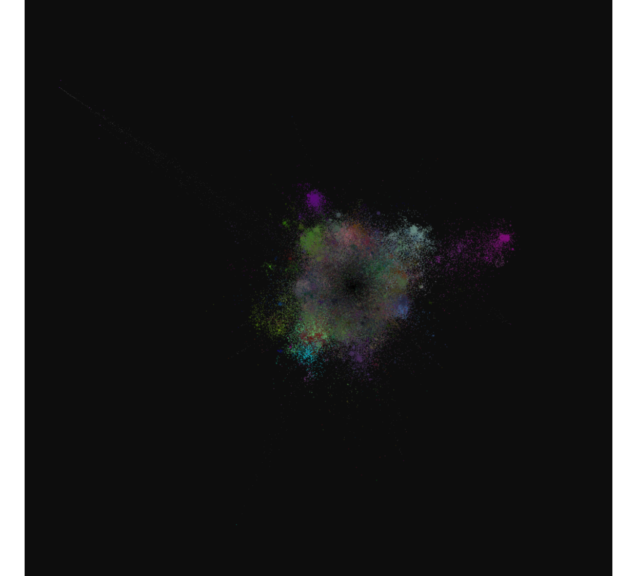
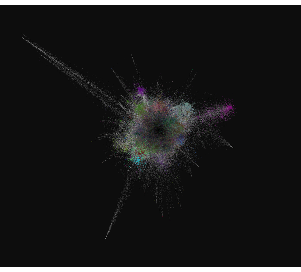
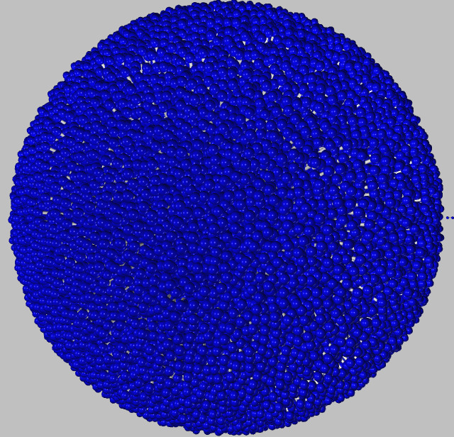
Treecapitator identifies some high-degree hubs (major web portals) and separates them from the dense low-degree majority, but overall interpretability is limited. Graphia collapses everything into a blue mass — essentially unreadable.
Catalan Linguistic Dependency Graph
Derived from the syntactic dependency trees of Universal Dependencies, AnCora Catalan corpus. Each unique token is a node; two nodes are connected if there is any syntactic dependency between their tokens in the corpus.
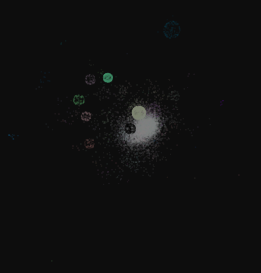
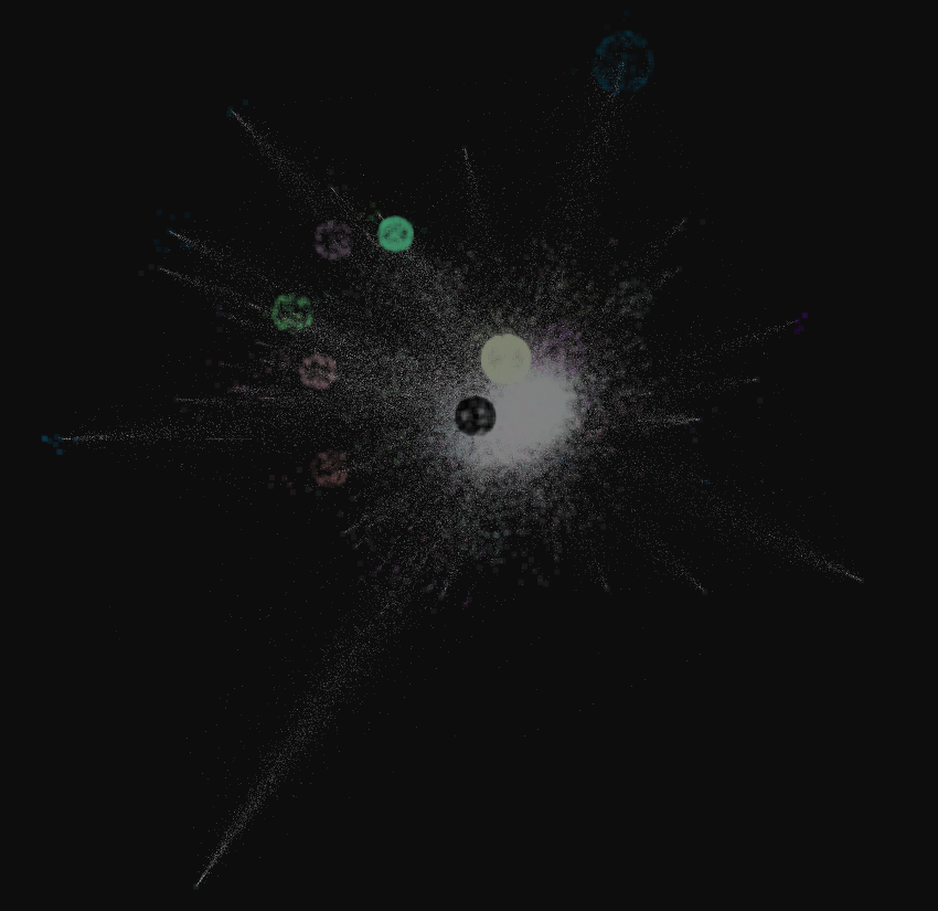
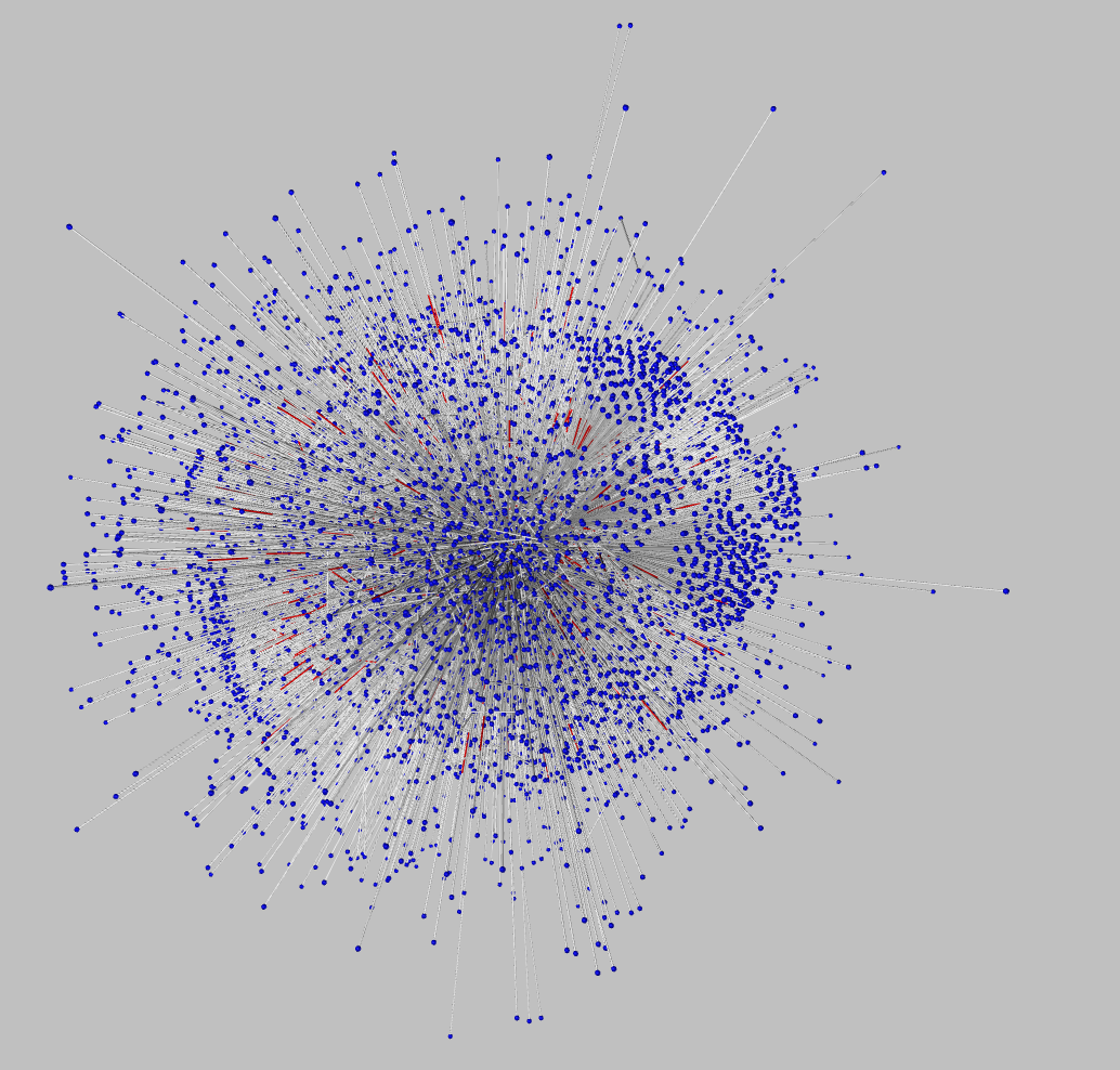
The linguistic graph has a high average degree (15.91) and a mix of very-high-degree function words (articles, prepositions) and low-degree content words. Treecapitator produces small satellite clusters analogous to the email case, though with less clear separation. Graphia shows a similar clustering tendency.
Parameter Study
Parameter b — Overall Scale
controls the radius of the sphere within which hubs are scattered ( throughout). Increasing expands the layout proportionally. The relevant quantity is the ratio : when every node collapses toward its neighborhood; the jitter dominates and the layout degenerates.
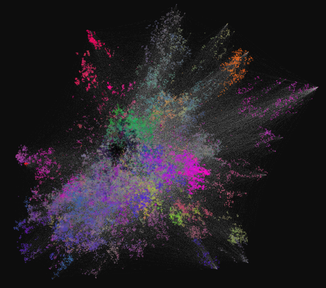
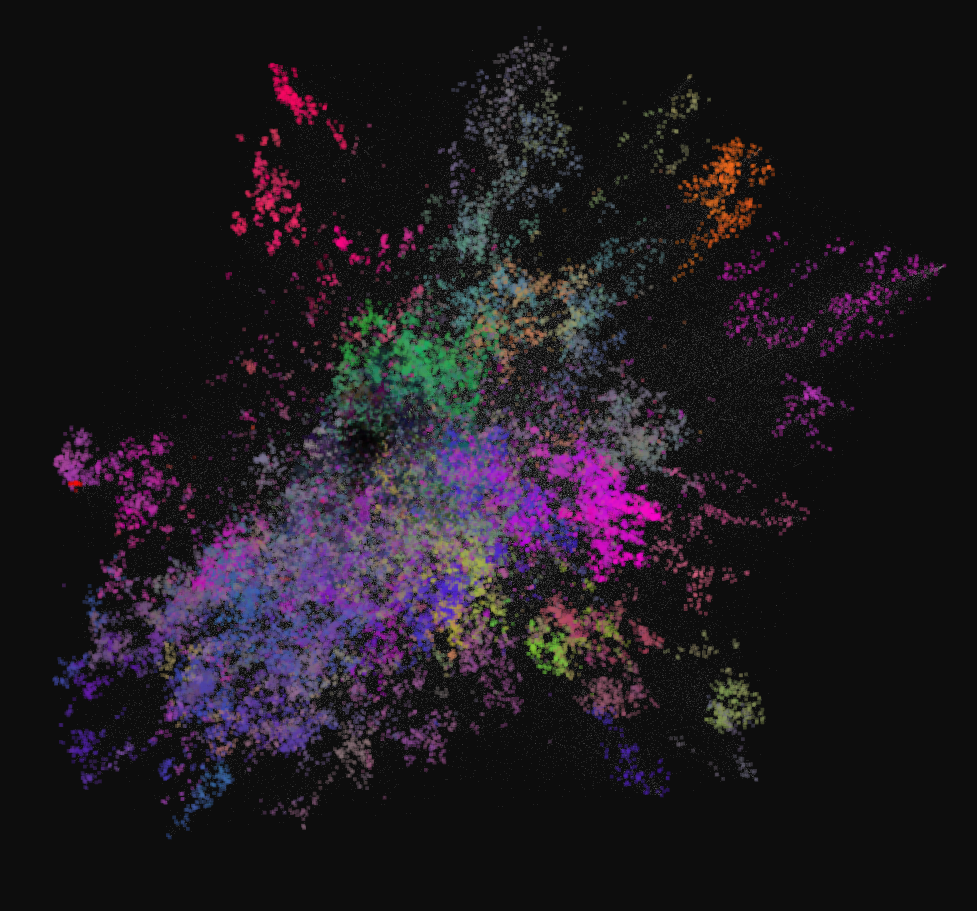
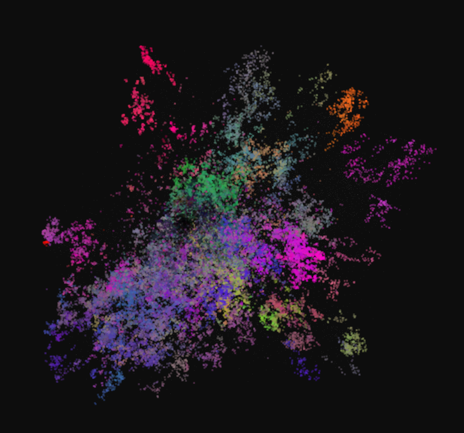
BA network (50k nodes) with b ∈ {2, 10, 100}. Scale has been normalized for comparison; the structural shape remains stable — b primarily controls the radius and therefore the visual density.
Parameter c — Jitter / Bubble Separation
controls the influence of : it prevents collapse of nodes with identical adjacency lists. Its most visible effect is on the Factor Graph model, where many nodes share the exact same neighbor set due to the deterministic divisibility rule.
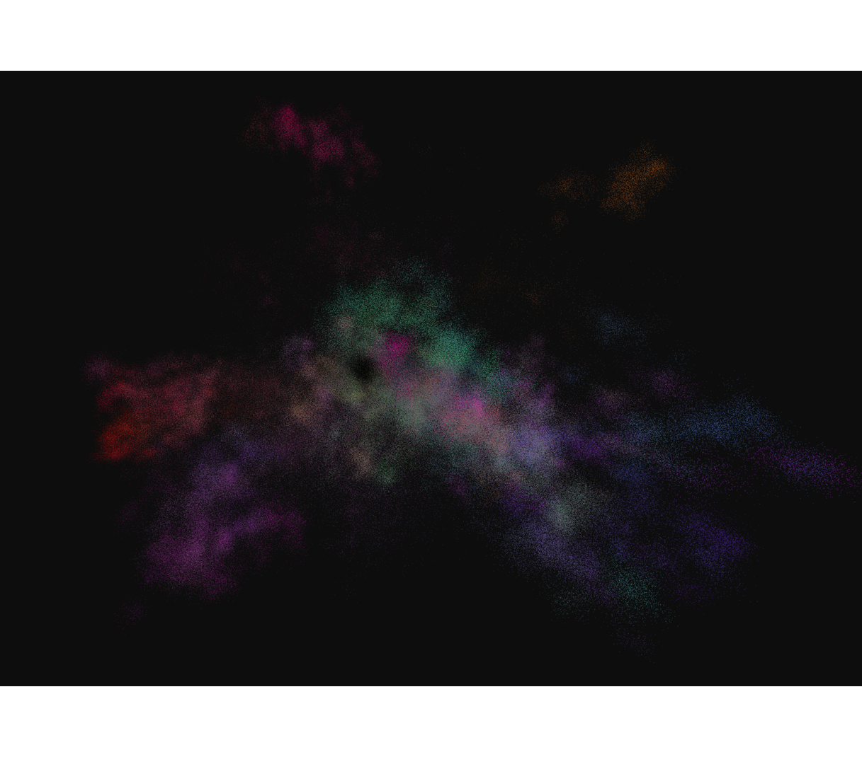
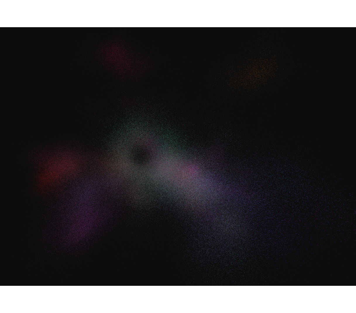
BA network (10M nodes) with c ∈ {0, 1.358, 4.482}. Increasing c blurs the network by distributing nodes away from their structural position — at high c the layout degenerates into a uniform cloud.
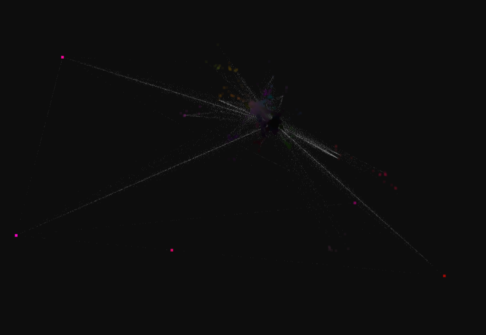
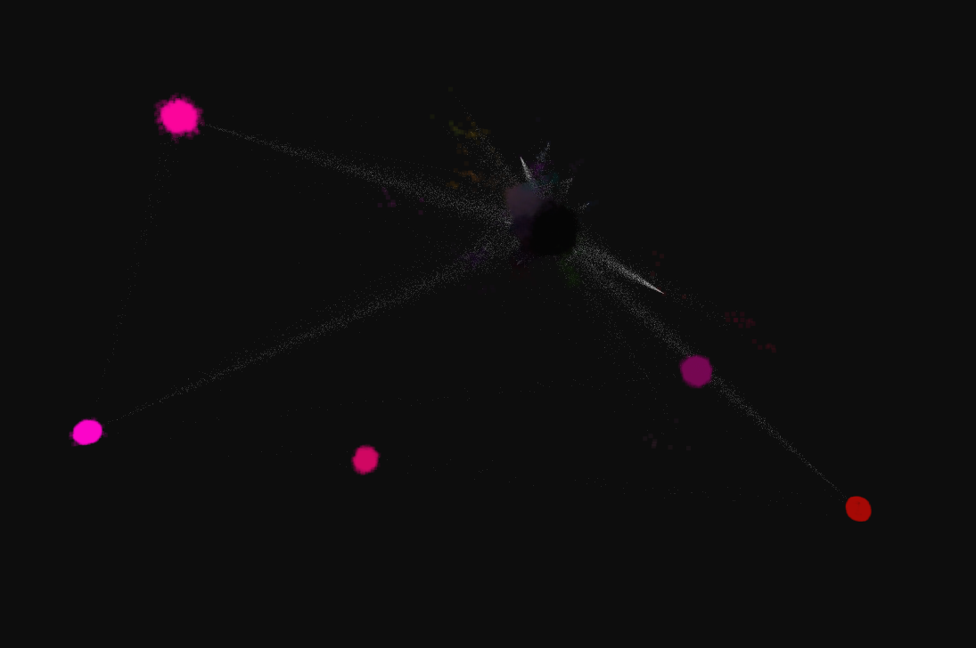
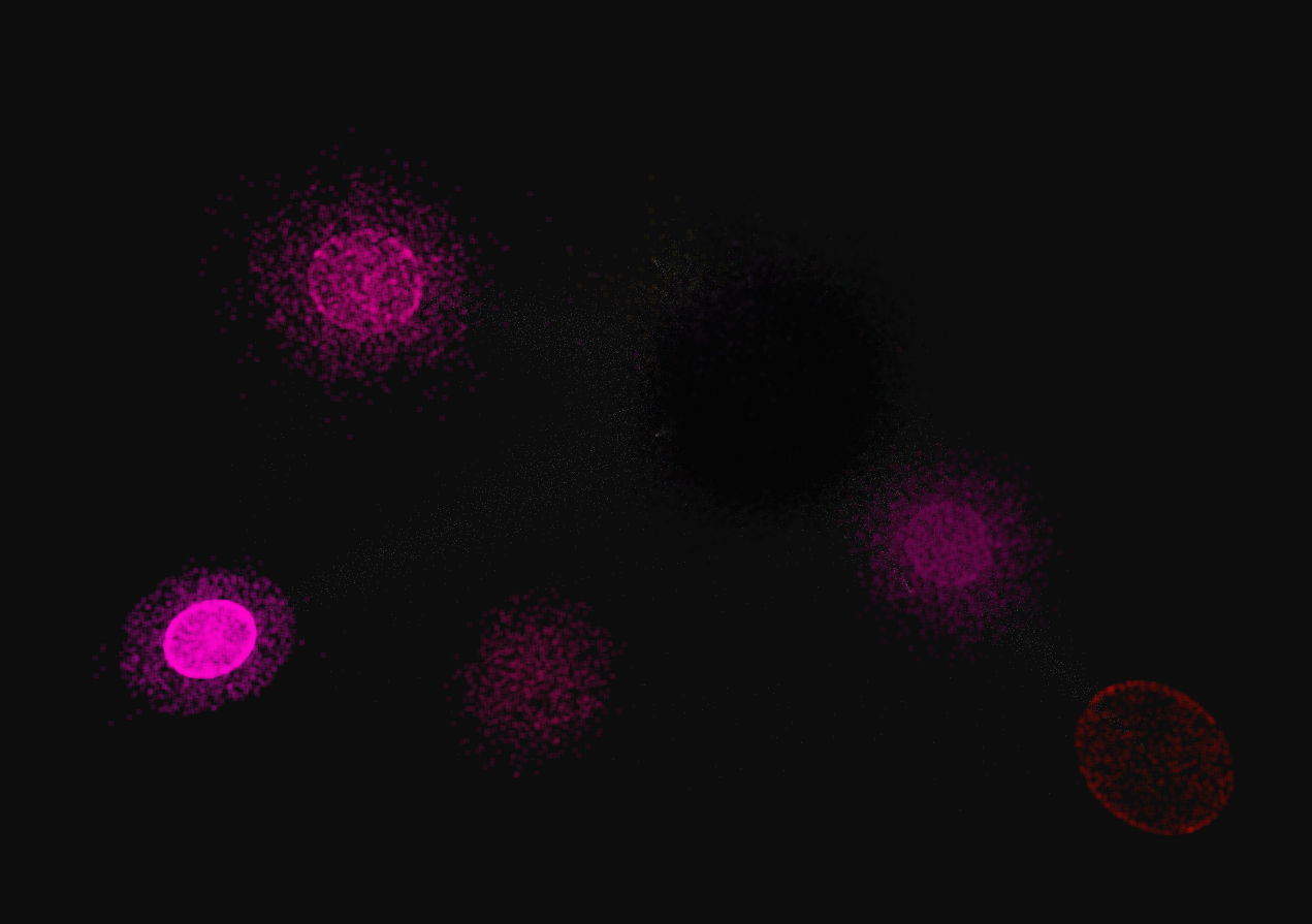
Factor Graph (150k nodes) with c ∈ {0, 1.094, 6.218}. The bubble clusters (groups of nodes sharing the same adjacency list) remain distinctly separated by jitter c. At c=0 they are point-like; increasing c expands the bubbles while preserving the inter-bubble structure.
Parameter τ — Softmin Temperature
controls how greedy the placement is. At , softmin degenerates to argmin and every node is placed exactly at the position of its lowest-degree hub neighbor. At higher , the selection softens across the neighborhood.
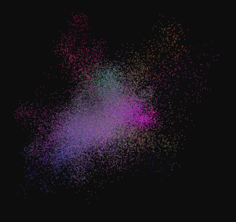
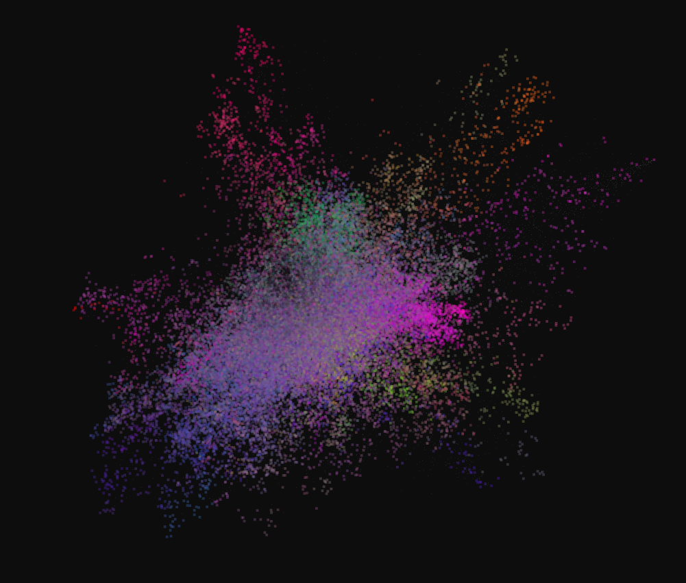
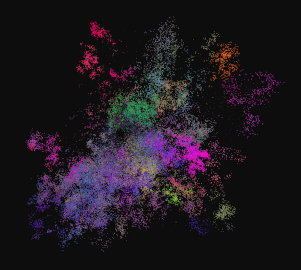
BA network (50k nodes) with τ ∈ {4, 1, 0}. At τ=0 the fractalized, self-similar structure of the Barabási–Albert model becomes most apparent — the layout acquires a characteristic branching pattern. This is one of the more visually striking results of the algorithm.
The τ=0 result on BA networks reveals a self-similar structure that may relate to the fractal dimension of the network's degree sequence. Quantifying this precisely with a box-counting algorithm is left as future work.
Rendering Parameters
Alpha Blending
Alpha blending is the single most important rendering parameter for dense graphs. Without it, overlapping node points form an opaque wall; with it, the local density of nodes is directly visible as brightness.
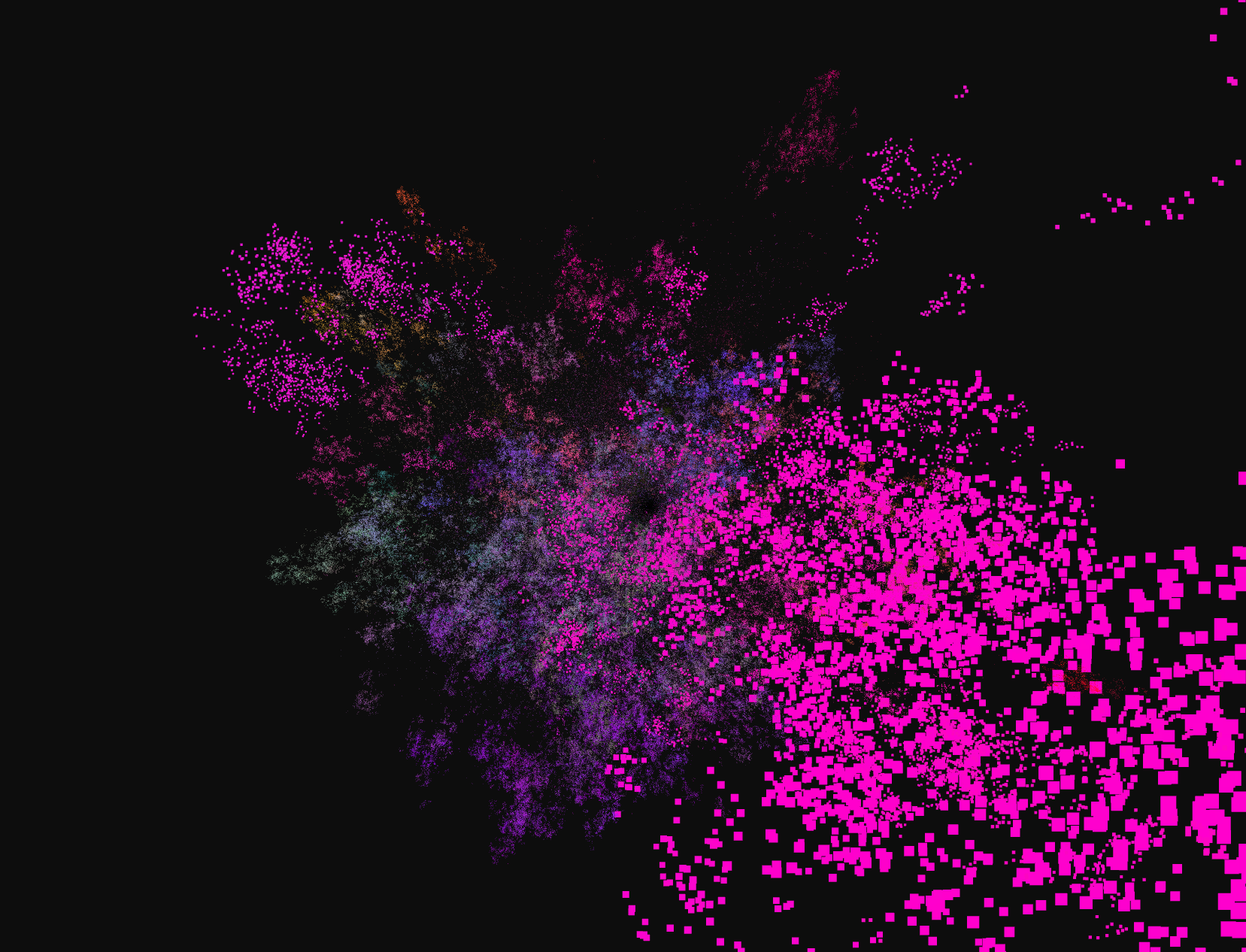
Alpha ∈ {0.11, 0.50, 1.0}. Low alpha reveals internal density structure. Full opacity hides it. For graphs with millions of nodes, α ≈ 0.1 is typically the most informative.
Edge Thickness
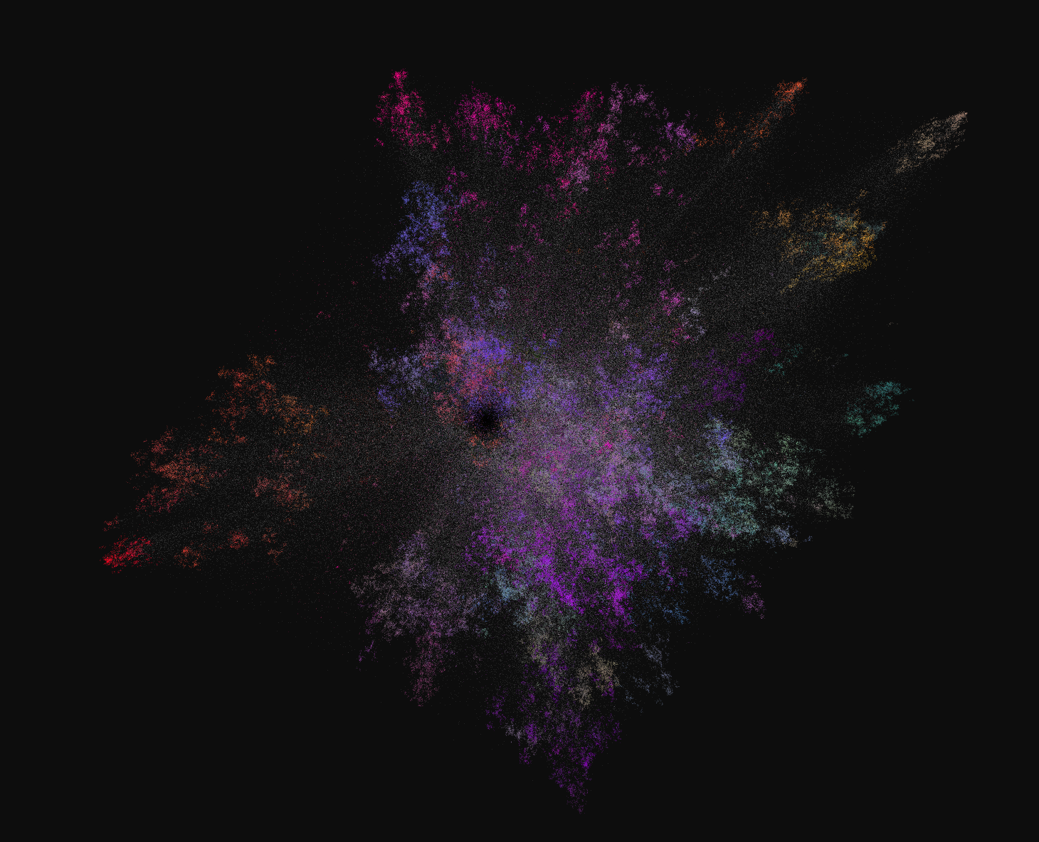
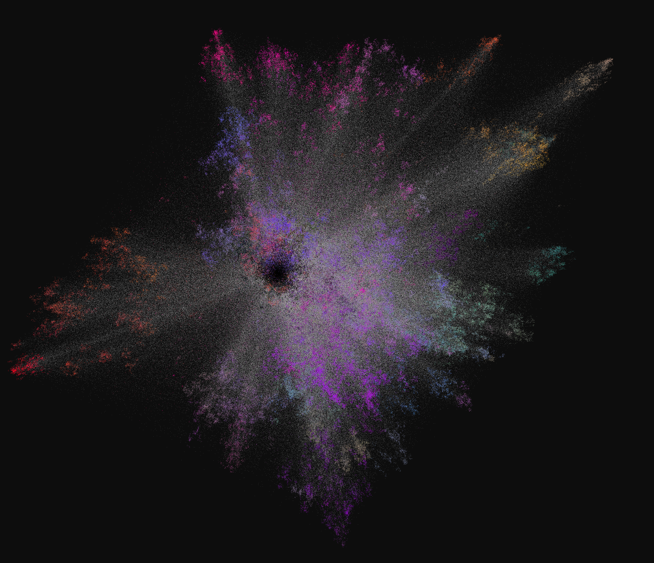
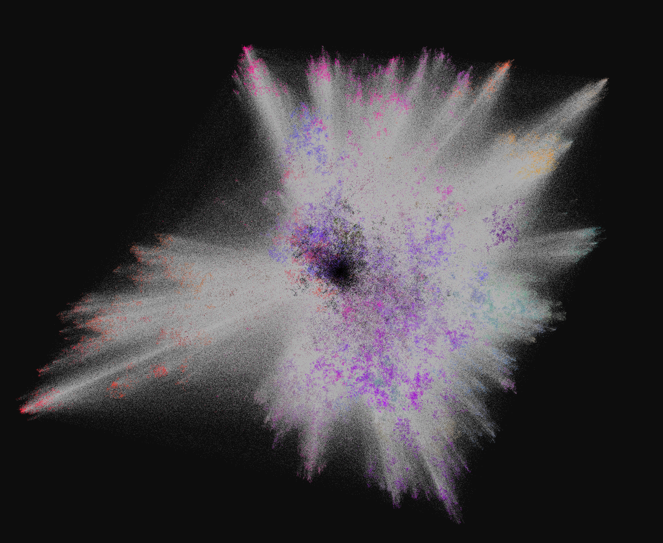
Edge thickness ∈ {0.000018, 0.000064, 0.000598}. Edge rendering is most informative at low thickness on dense networks; thick edges saturate the render and obscure the node distribution. The optimal value is graph-specific.
Conclusions
RQ1 — Visual clarity for power-law graphs
Partially. The email, WebGraph, and linguistic networks show meaningful interpretable structure. Road networks are completely opaque to this approach. The layout is most informative for graphs with a strong power-law degree sequence and a mix of very-high and very-low degree nodes.
RQ2 — Usefulness
Limited, but interesting. The algorithm creates visually distinctive forms for Barabási–Albert and Watts–Strogatz networks and reveals "bubble" communities (collections of nodes connected to exactly one hub). On natural networks the utility is still quite lacking, though it provides a unique way to see connectivity relationships between nodes not present in standard tools.
RQ3 — Behaviour on non-power-law graphs
On graphs that do not follow a power-law degree sequence (tested on ER binomial), Treecapitator produces spheres of varying thickness as a function of average degree — an honest representation of degree uniformity with no false structure imposed.
RQ4 — Improvement over stock algorithms
Minimal improvement is observed for WebGraph and Barabási–Albert, where the algorithm produces a more legible layout than Graphia's force-directed approach. For road networks the algorithm offers nothing useful; the geographic structure captured by force-directed methods is significantly more informative.
RQ5 — Parameter sensitivity
- is a scaling constant; the relevant quantity is . Its shape effect only appears at extreme values.
- only meaningfully impacts networks with high numbers of nodes sharing the same adjacency list (Factor Graph model). For other graphs, gives the clearest result.
- is the most structurally significant parameter for Barabási–Albert networks. Setting reveals a self-similar fractalized layout. For all other tested networks, should be set near 0 for clearest results.
Final Assessment
This model is visually compelling and provides a fast layout algorithm, but it fails to efficiently lay out and render large power-law graphs with competitive interpretability relative to established tools. It is not a replacement for Graphia or similar force-directed systems on most real-world graphs.
Its most interesting results are in the study of synthetic graphs that follow Barabási–Albert structure, where the fractalized layout at and the bubble organization of the Factor Graph reveal structural properties not visible in conventional layouts. These remain open questions for further study.
Implementation
The visualizer is implemented in C++ with OpenGL, using CMake as the build system. It accepts graph data as edge-list pairs in plain text or compressed Gzip (SNAP format) and CoNLL-U dependency files (which it aggregates into a graph automatically).
Data validation is built in: the tool displays node-count and edge-count statistics alongside degree plots in both linear and log scale, making it straightforward to verify that the algorithm is correctly placing higher-degree nodes as described.