Immediate Radiosity
A real-time global illumination pipeline based on precomputed radiosity, implemented entirely on the GPU using Vulkan compute shaders.
Results
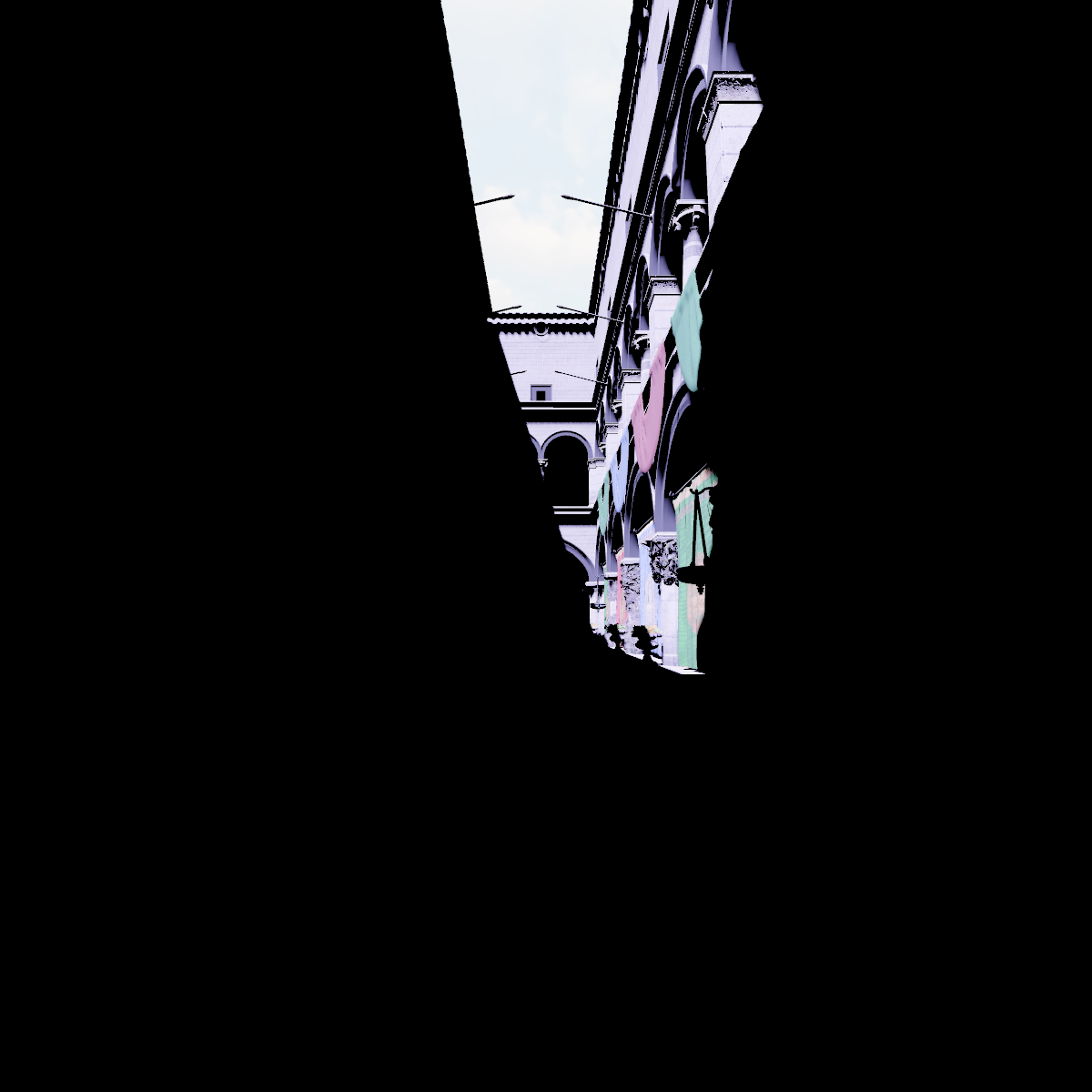
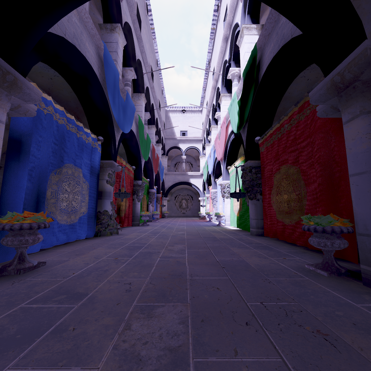
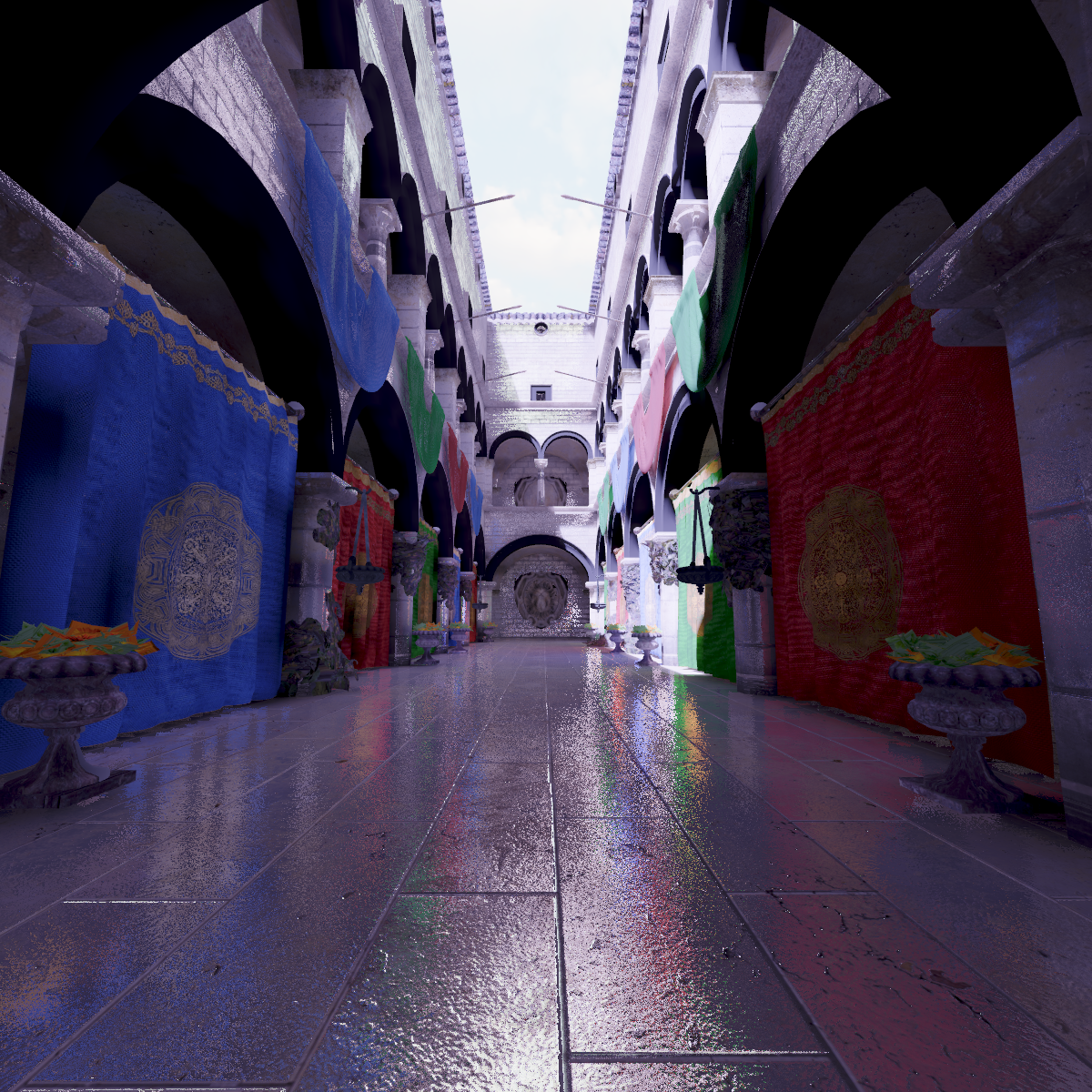
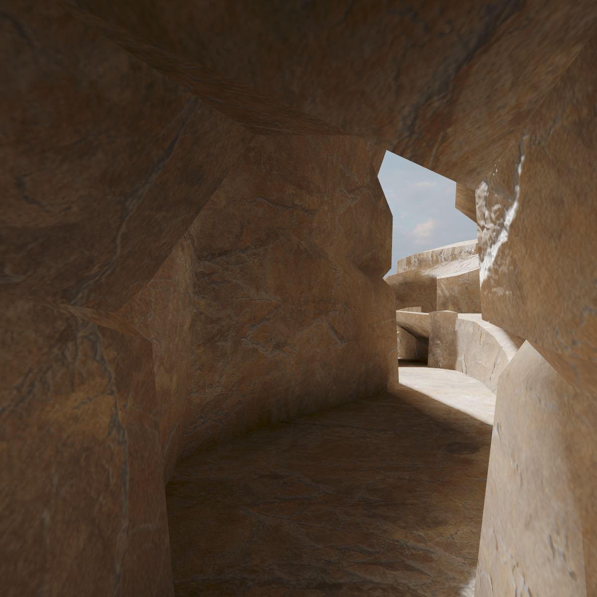
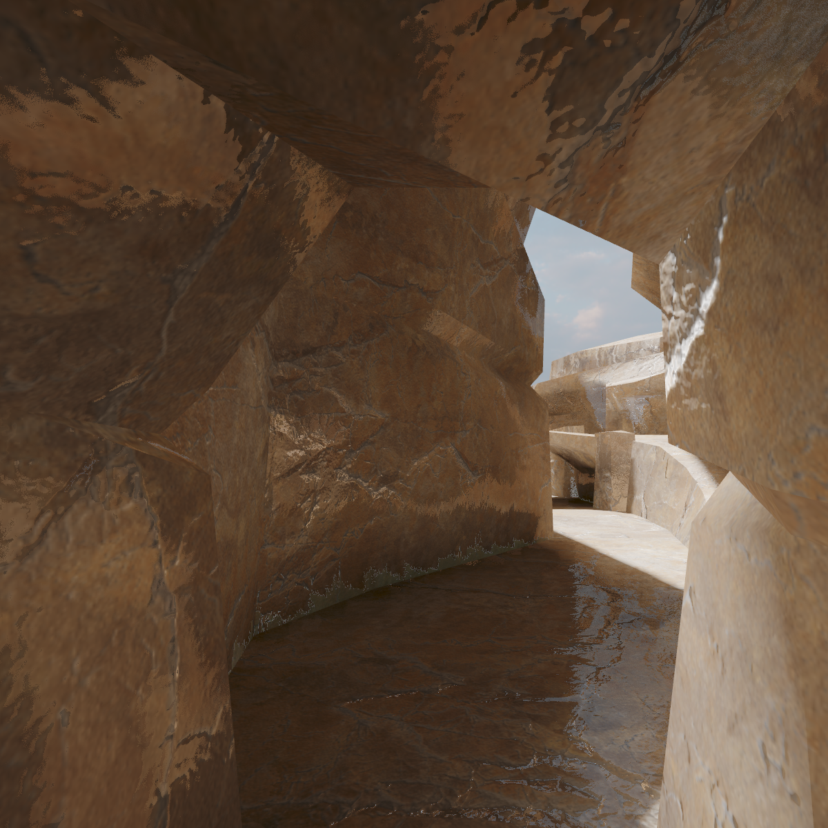
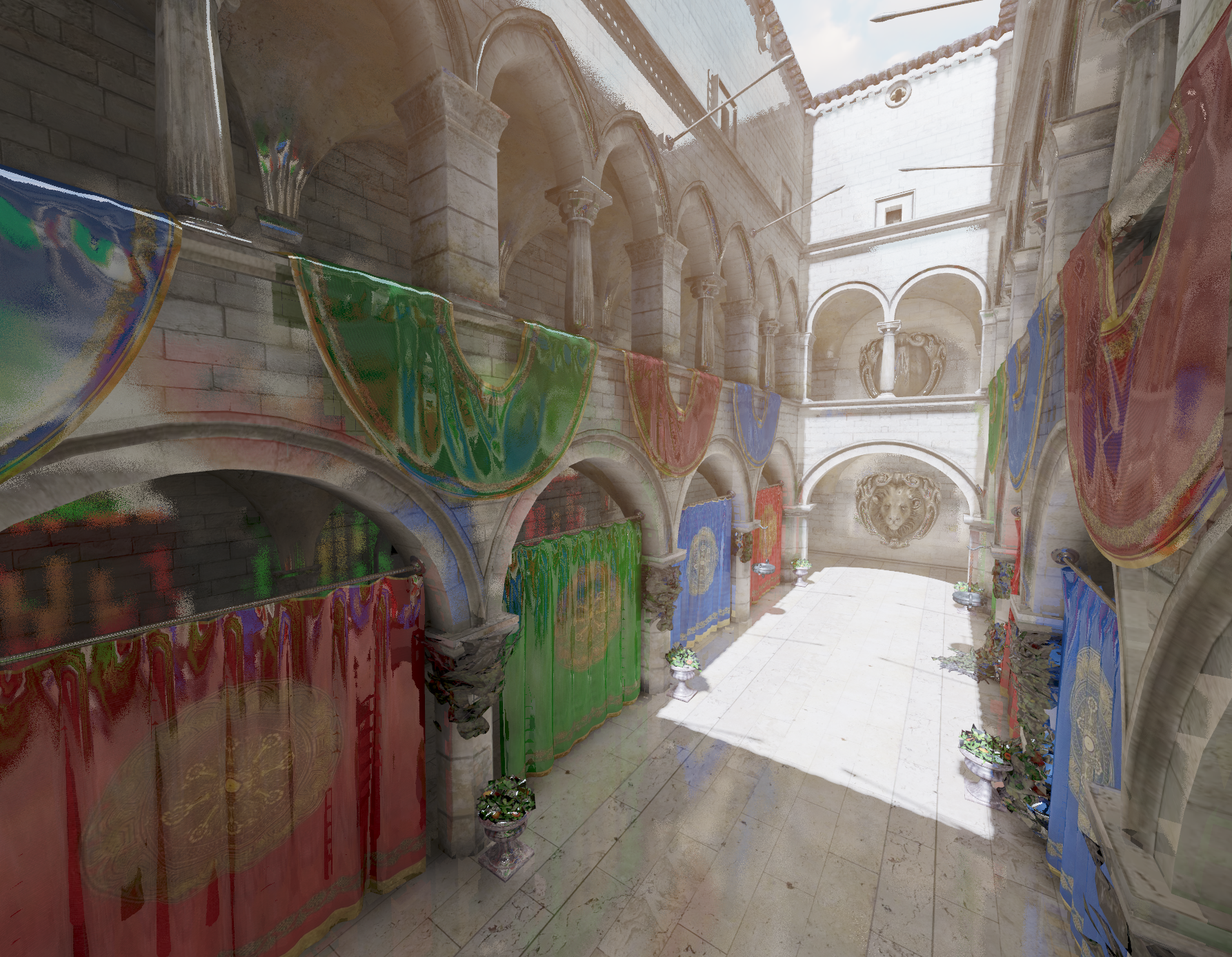
The following renders show the system running on four test scenes. Each row compares the same viewpoint rendered without global illumination, with diffuse GI only, and with the full pipeline (diffuse + specular indirect).
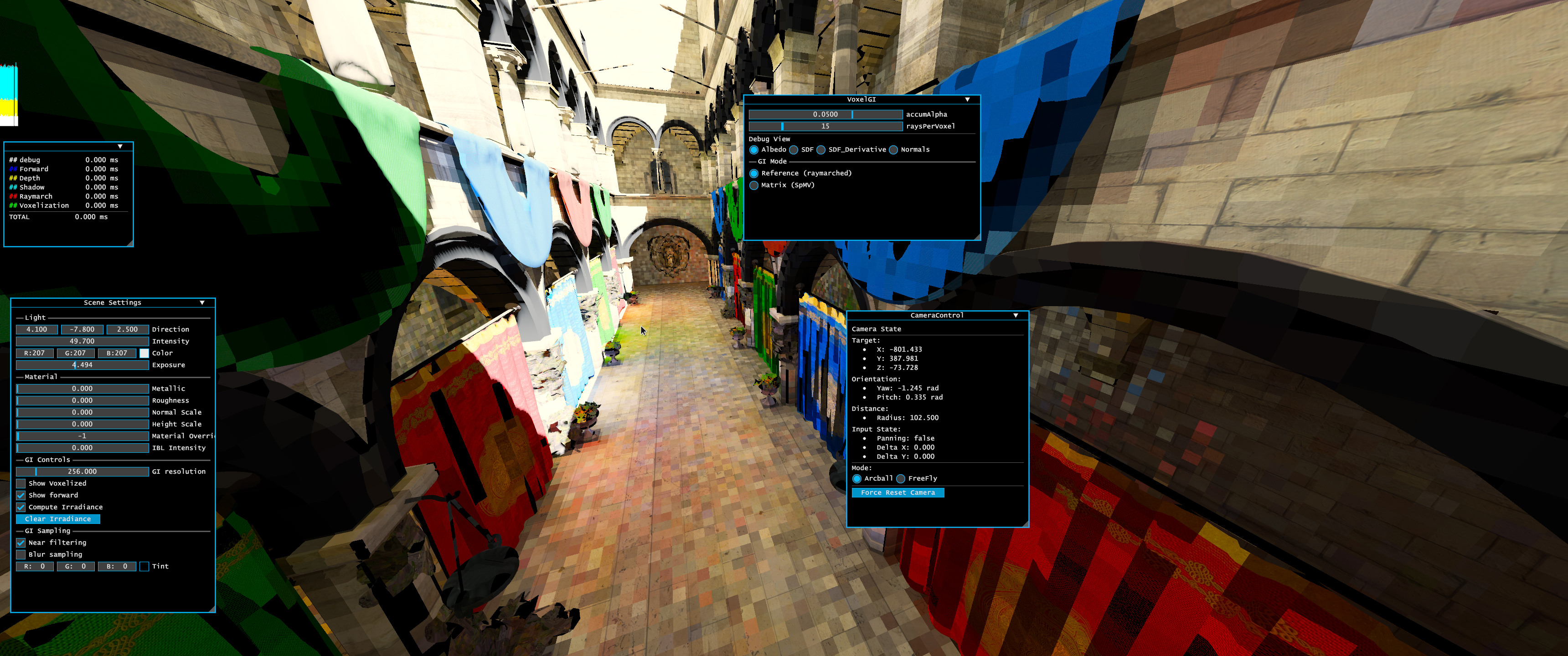
Sponza:
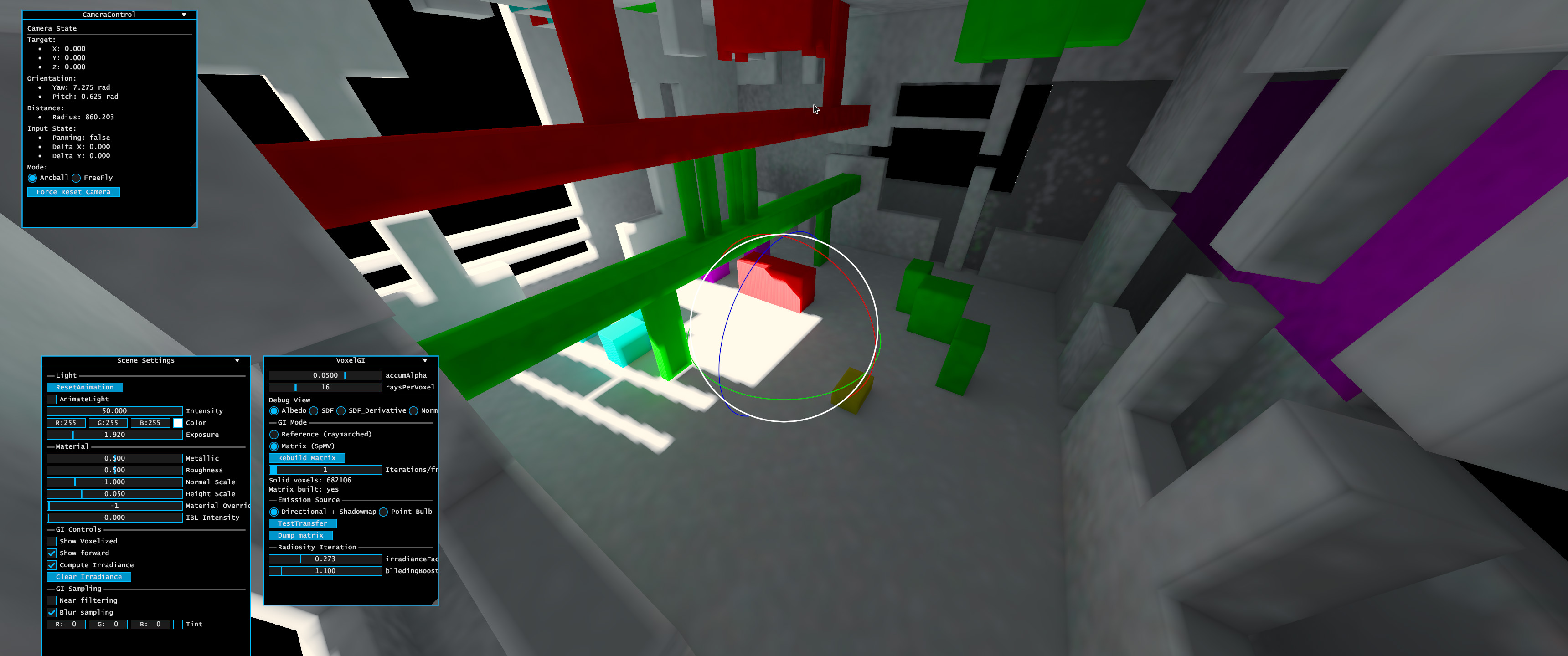
Box (Cornell-like scene with curved geometry):
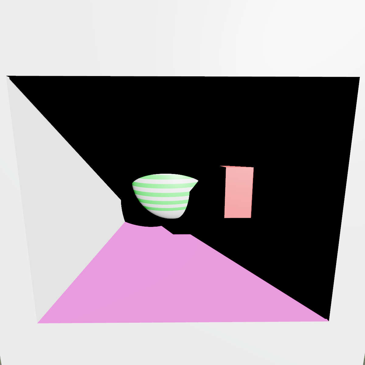
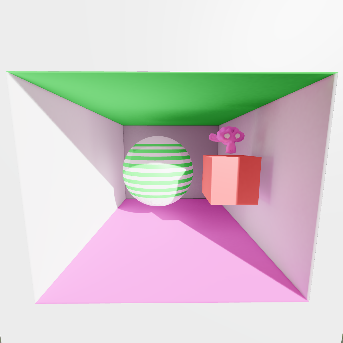
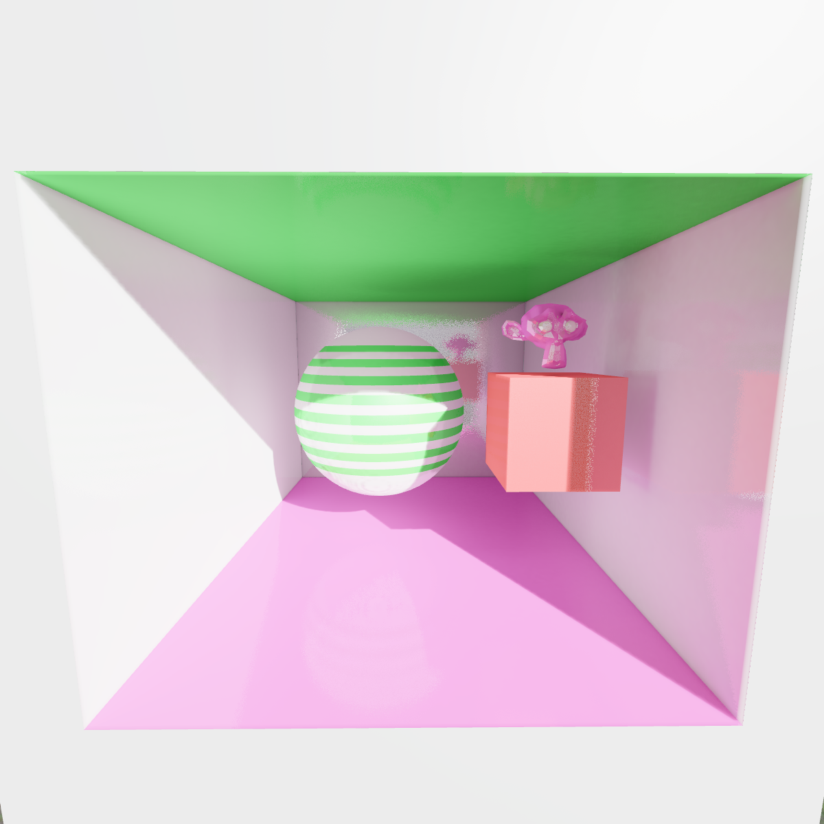
Arena (cave/desert scene):
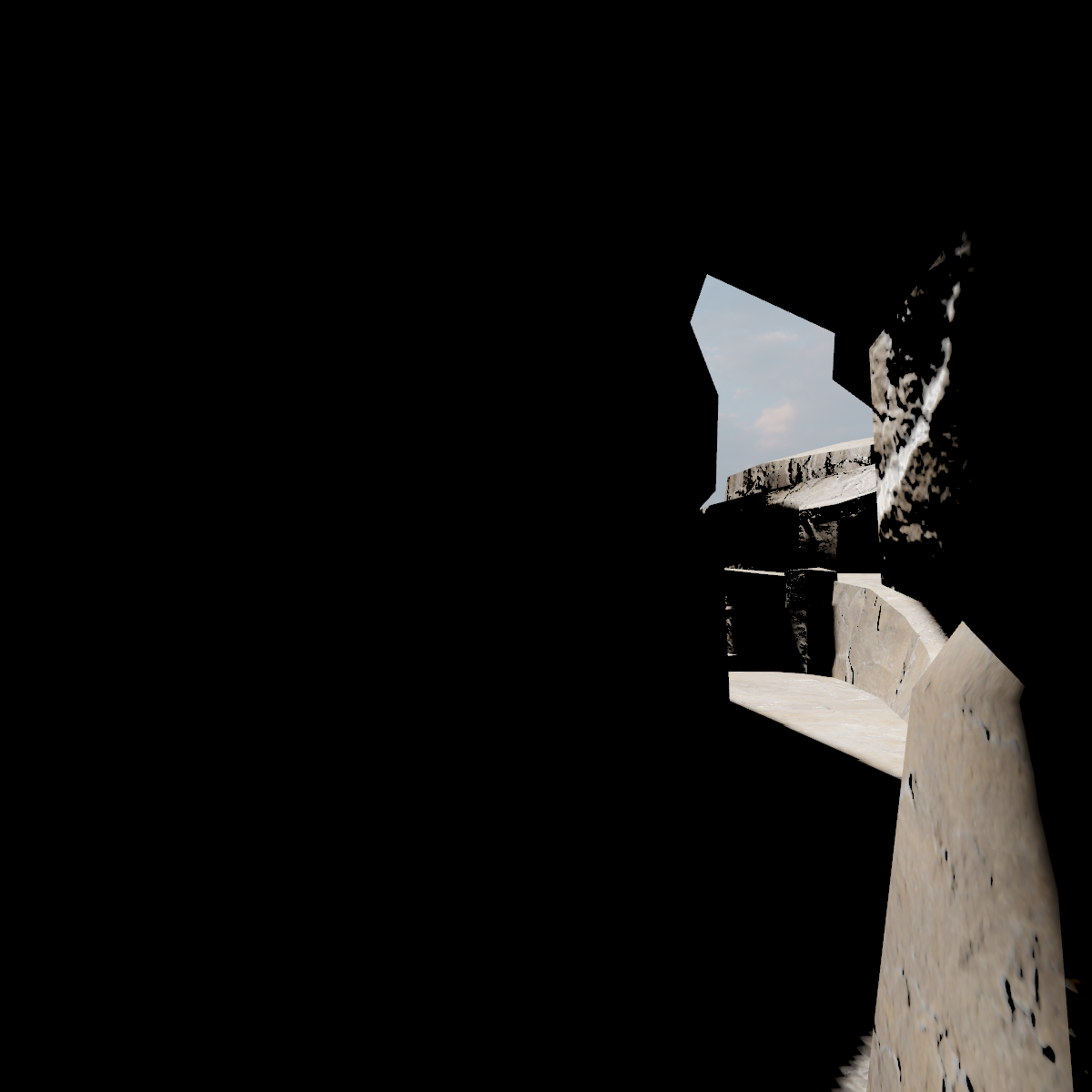
Abstract Park (multi-surface light bounce test):
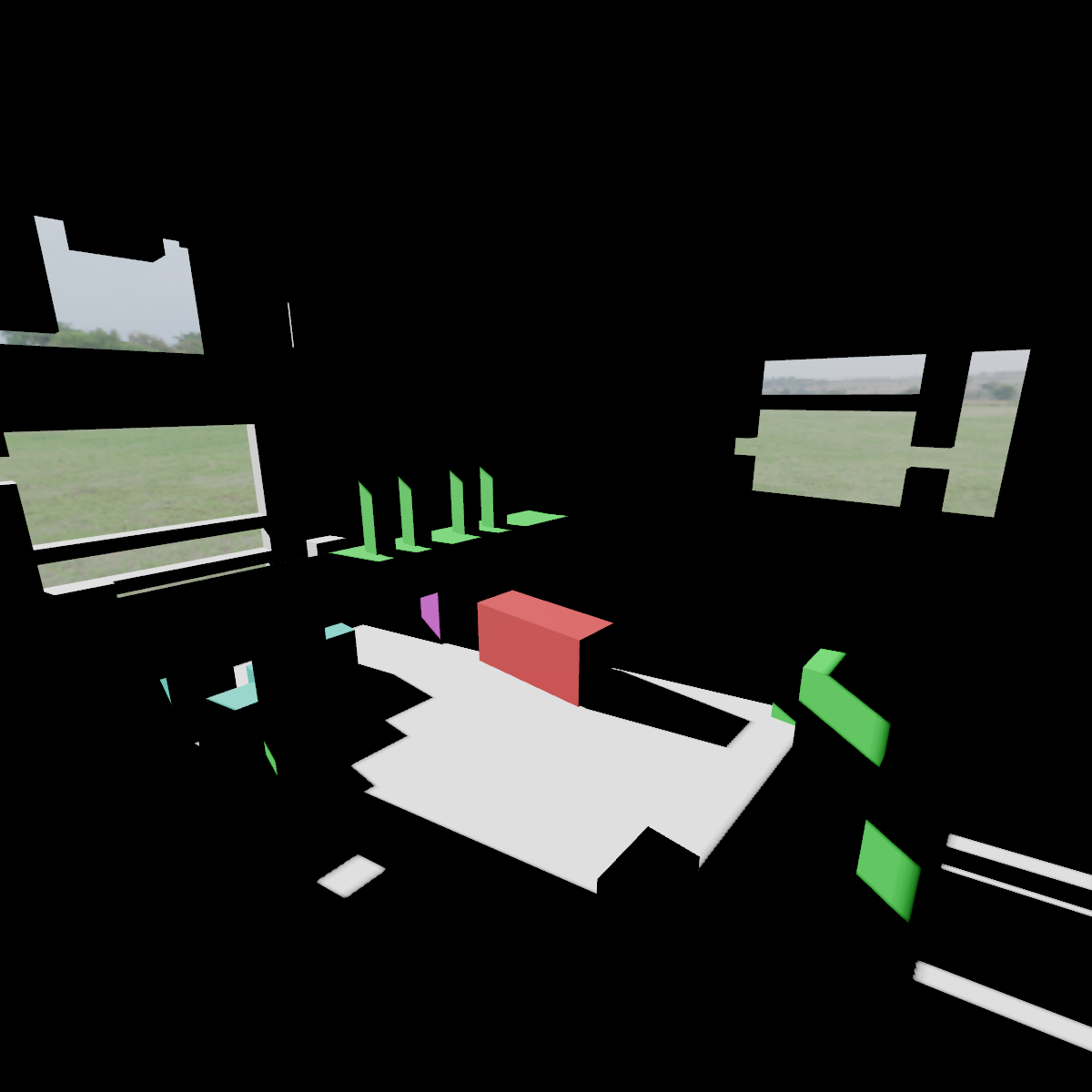
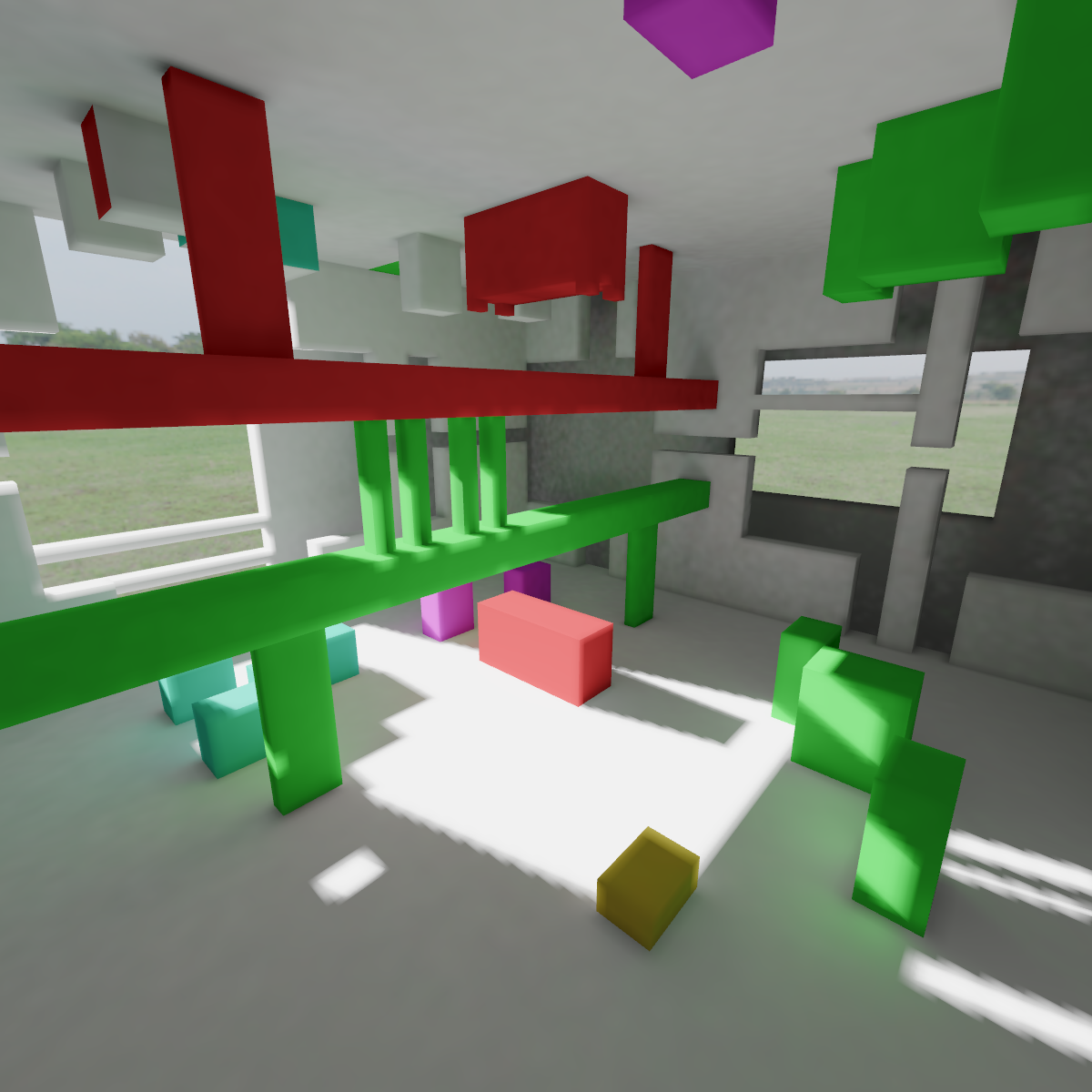
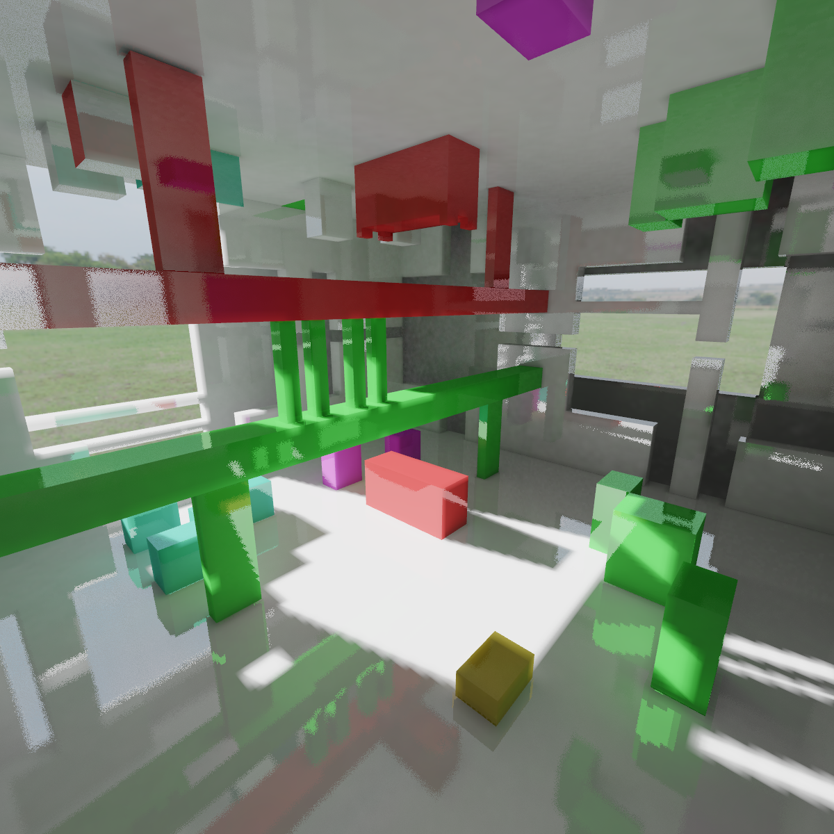
Each triplet: no GI (left), diffuse GI only (center), full GI with specular indirect (right).
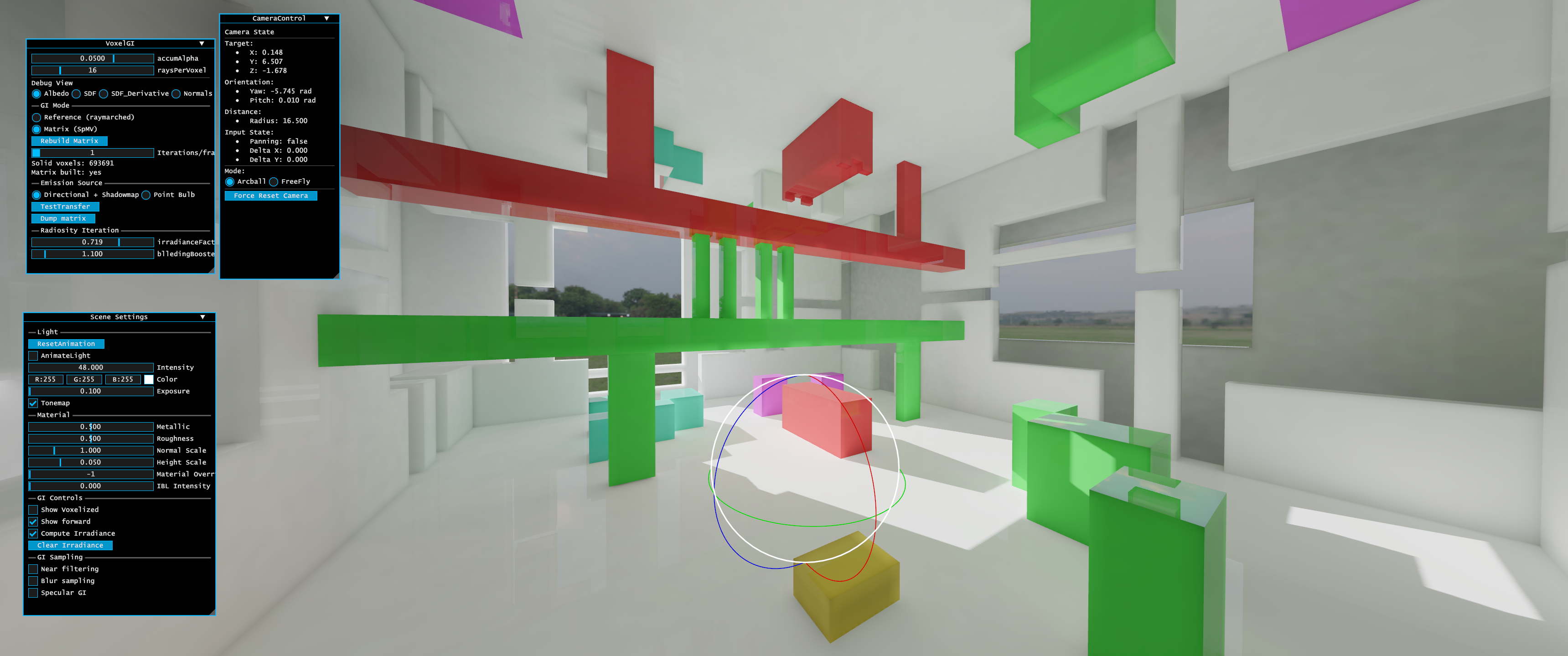
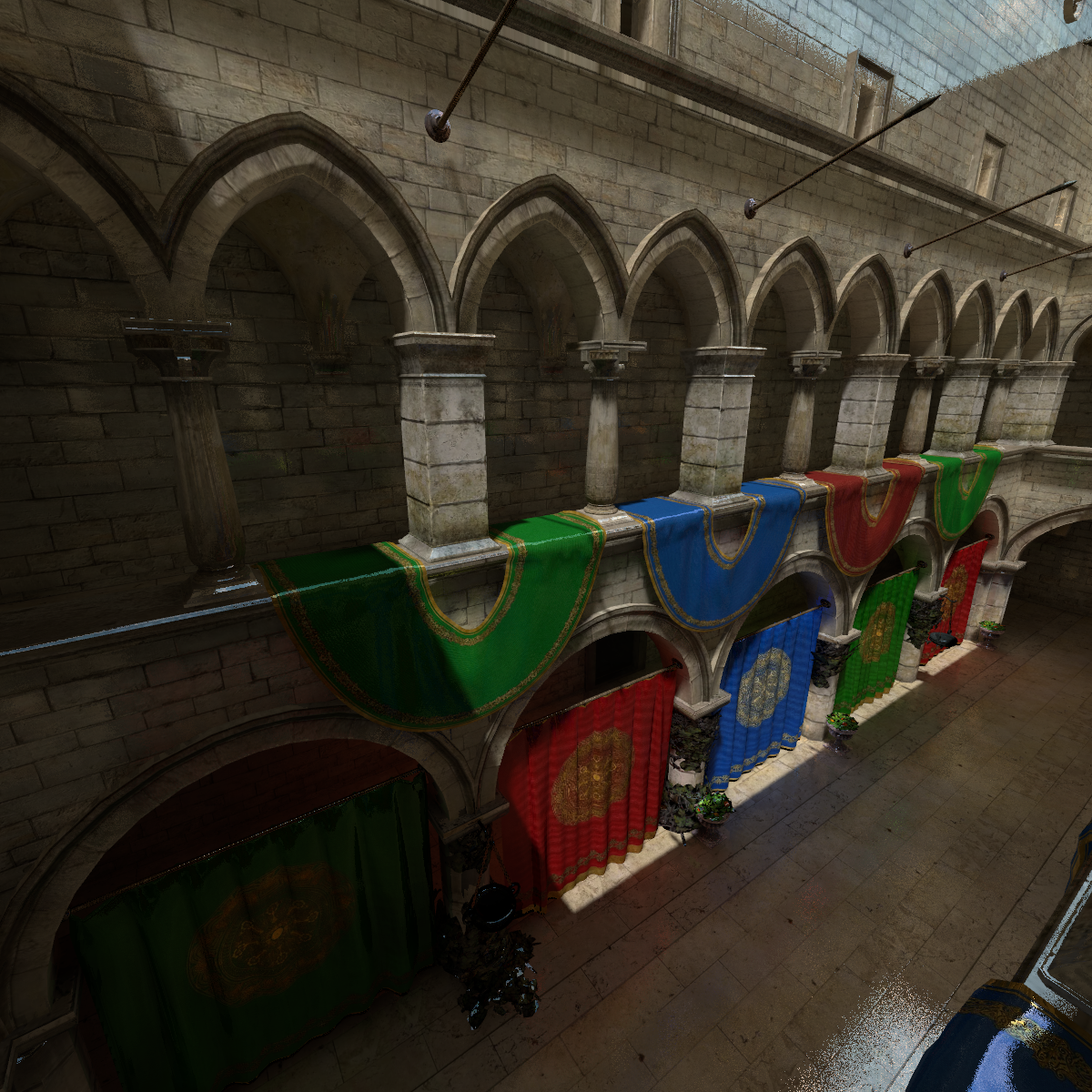
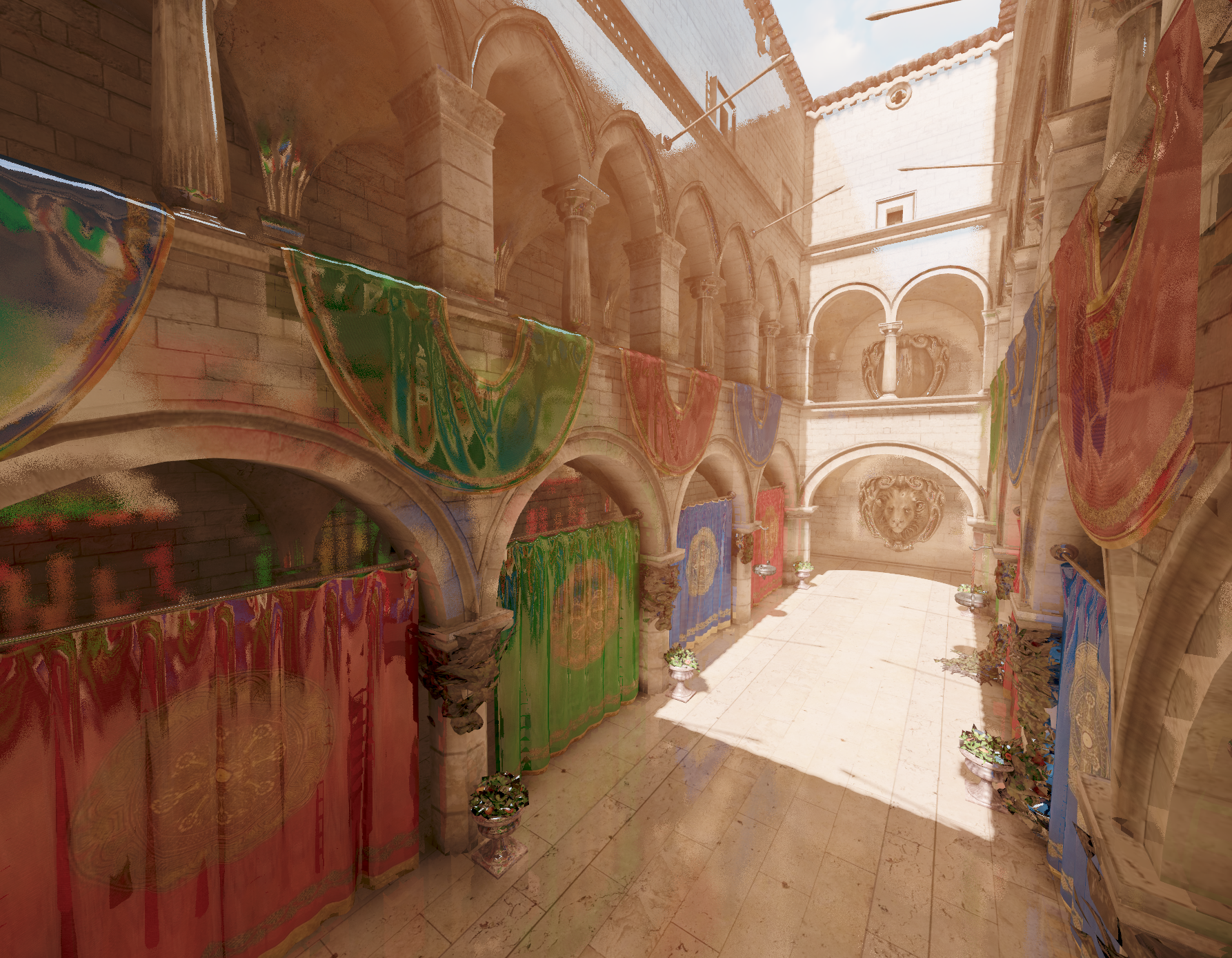
GI Component Decomposition
The forward shader composites the final image from diffuse and specular indirect contributions, each sampled independently from the radiance volume. Here is the decomposition for the Sponza scene:
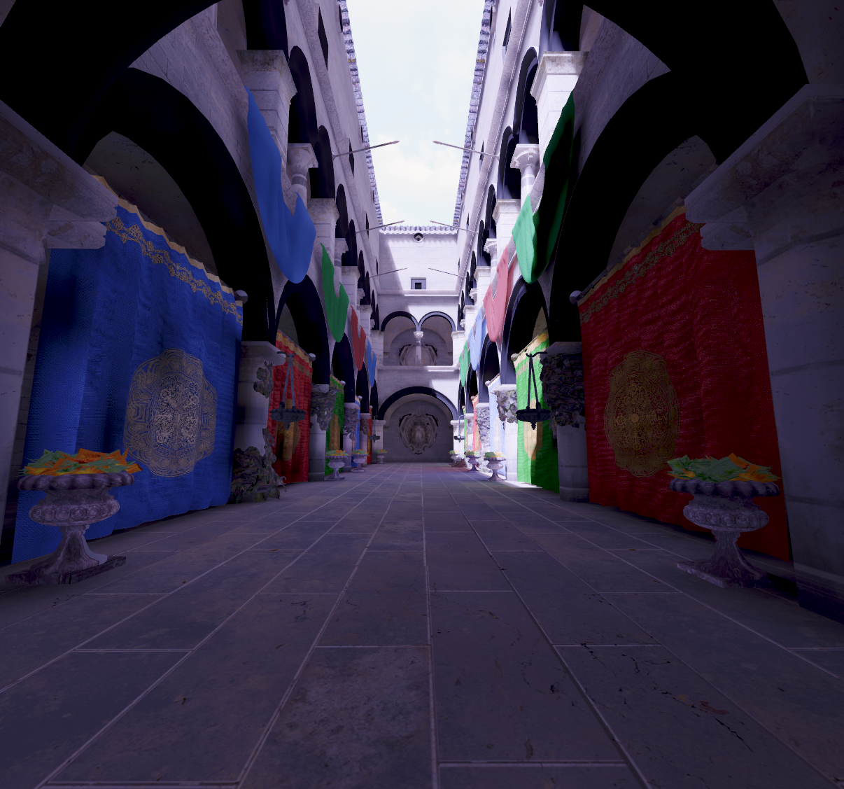
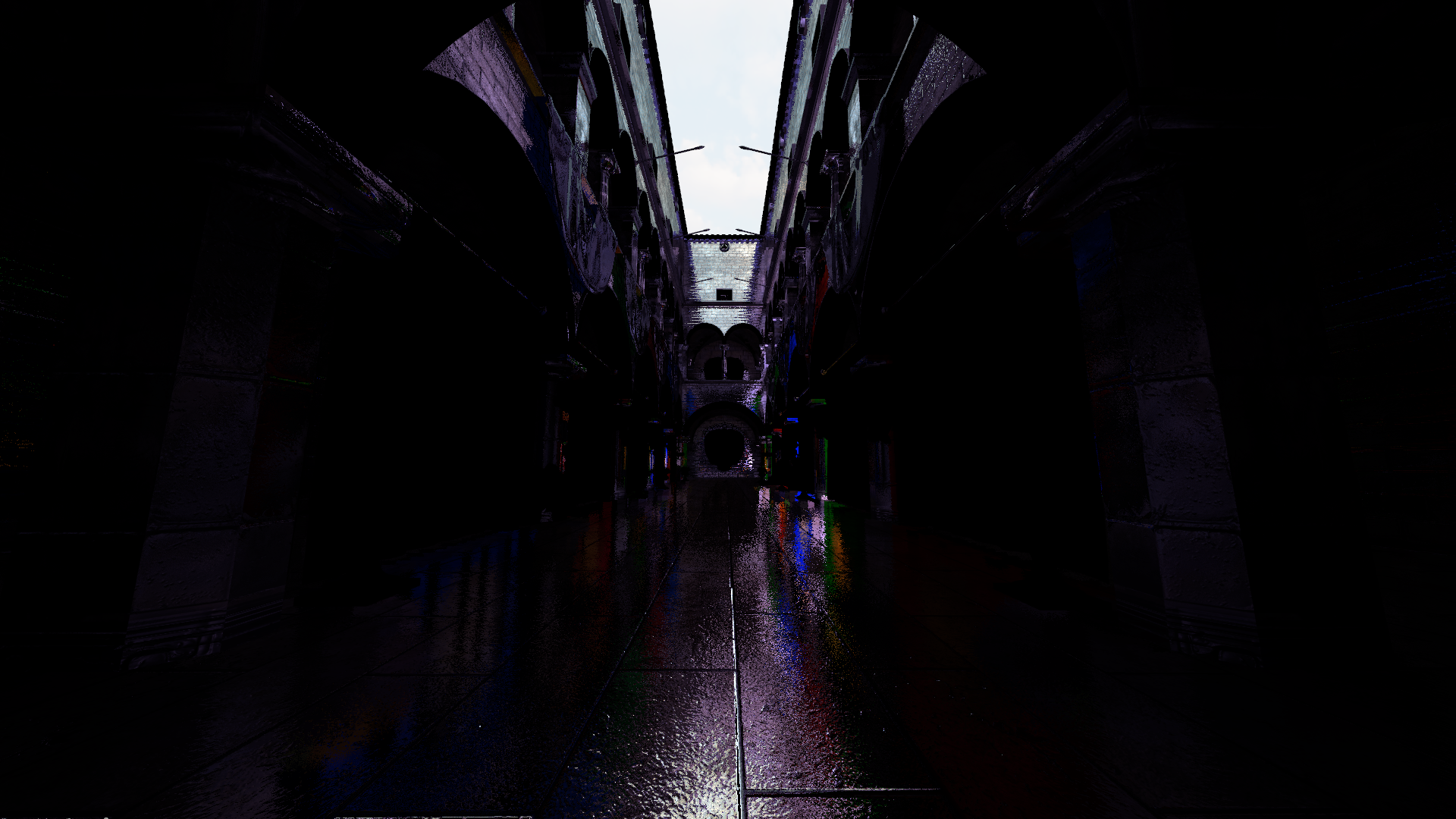
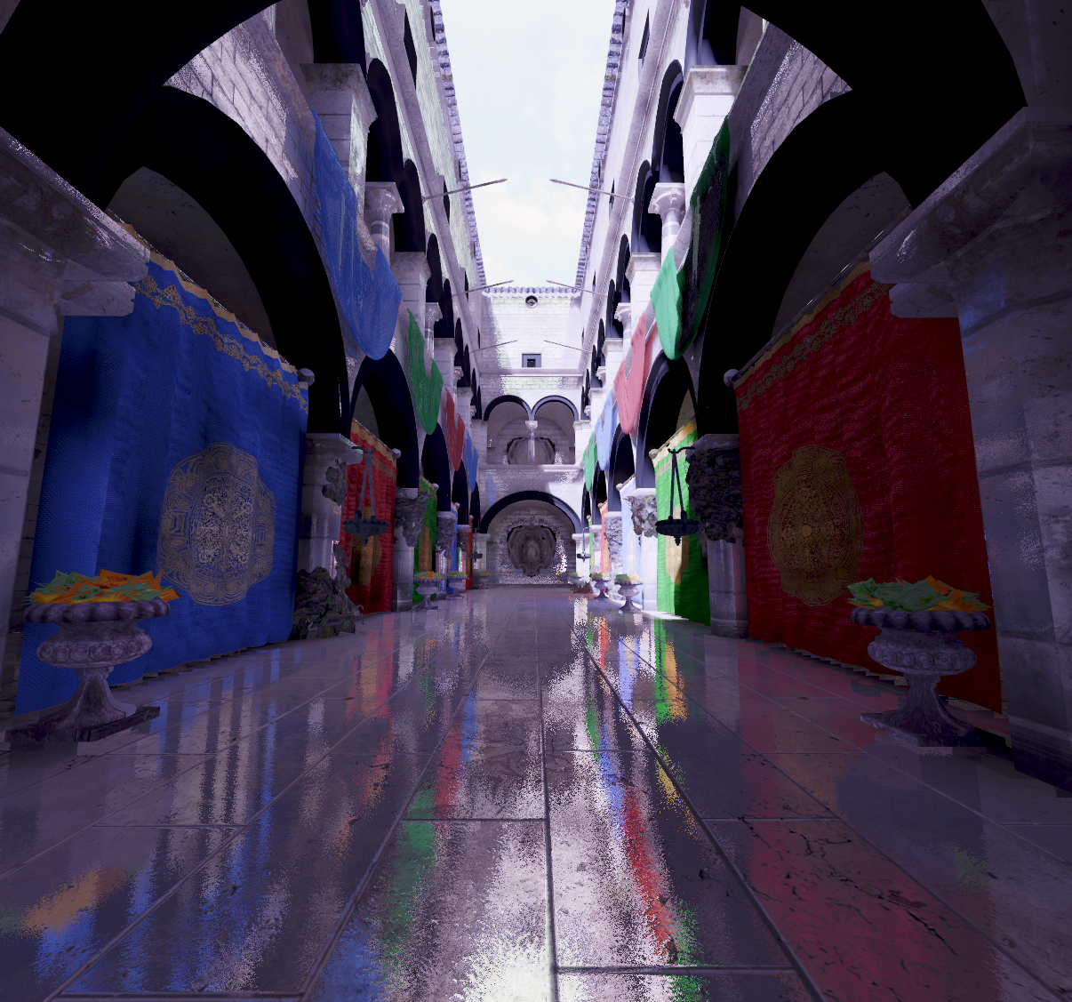
Left: diffuse indirect (sampled from the radiance volume). Center: specular indirect (raytraced through the voxel volume). Right: full composite with PBR coefficients.
Demos
Key Performance Numbers
| Metric | Value |
|---|---|
| Per-frame relight (SpMV) | 2–4 ms on AMD RX 7700 XT |
| Matrix construction (Sponza, , DDA) | ~10 s (one-time) |
| Matrix construction speedup with SDF | ~2× faster |
| GPU memory (Sponza, , ) | 3 287 MiB |
| Solid voxels at (Sponza) | 441 511 |
Introduction
Real-time global illumination remains one of the central unsolved problems in interactive rendering. Commercial engines approximate indirect light through a combination of voxel cone tracing, screen-space techniques, and radiance caches, but all of these approaches share a common cost: some form of ray traversal must occur every frame, either through hardware ray tracing, voxel cone marching, or probe resampling. That per-frame traversal cost scales with scene complexity and imposes a hard budget that competes directly with the broader rendering pipeline.
This project investigates a different formulation. Radiosity expresses global illumination as a linear system over surface patches: the radiance of each patch is the weighted sum of contributions from all mutually visible patches, where the weights (the form factors, or view factors) encode inter-patch geometry and visibility. Crucially, the form factors depend only on scene geometry, not on lighting. If the scene is static, they can be precomputed once and stored as a sparse matrix. The per-frame cost then reduces to a single sparse matrix-vector product (SpMV), a well-understood linear algebra primitive that maps efficiently onto GPU compute pipelines.
The central hypothesis is: precomputing visibility into a sparse radiosity matrix and reducing the runtime GI problem to an iterative SpMV can produce a competitive real-time indirect illumination result at lower per-frame cost than ray-traversal-based alternatives.
Theoretical Background
The Rendering Equation
The theoretical foundation of all global illumination algorithms is the rendering equation, formulated by Kajiya (1986):
where is the outgoing radiance at surface point in direction , is emitted radiance, is the bidirectional reflectance distribution function (BRDF), is the incident radiance arriving from direction , and the integral is taken over the hemisphere centered on the surface normal .
The fundamental difficulty stems from the recursive nature of this equation: is itself the outgoing radiance of whatever surface is visible from along , making the full solution a system of coupled integral equations over all surfaces in the scene. Direct illumination truncates this recursion at one bounce. Global illumination algorithms differ in how they approximate or solve the full recursive integral.
Radiosity Formulation
Radiosity simplifies the rendering equation by restricting to purely diffuse surfaces. Under this assumption, outgoing radiance is independent of viewing direction, and the continuous integral reduces to a finite sum over discrete patches:
where is the radiosity (total energy per unit area leaving) of patch , is its emitted energy, its reflectivity, and the form factor from patch to patch . In matrix form:
The form factor encodes the fraction of energy leaving patch that arrives at patch , accounting for geometry, orientation, and mutual visibility. Since depends only on scene geometry, it can be precomputed once for static scenes. The per-frame cost then reduces to iteratively solving the linear system, which in this implementation is done via Jacobi iteration dispatched as a GPU compute shader.
Prior Work and Context
Radiosity algorithms were first introduced by Goral et al. (1984) and refined by Cohen and Greenberg (1985) through the hemicube representation for efficient form factor computation, and further by Cohen et al. (1988) through progressive refinement. These contributions established the backbone for subsequent industry systems. However, the complexity in patch count and the large memory requirements for the full form factor matrix made practical adoption limited. Stochastic ray-tracing lightmappers proved more popular due to their flexibility and better scalability.
Geomerics Enlighten (later acquired by ARM and integrated into Unity and Unreal Engine) is the closest prior work. It also decouples expensive visibility computation from per-frame energy propagation, reducing runtime cost to a sparse matrix-vector product. However, Enlighten operates at a coarse patch resolution dictated by lightmap texel density and encodes only diffuse-to-diffuse (D→D) energy exchange. Specular indirect contributions are approximated separately through reflection captures rather than being derived from the transport matrix itself.
Voxel Cone Tracing (VCT), introduced by Crassin et al. (2011), represents the principal alternative for dynamic scenes. Commercial adaptations include NVIDIA VXGI (integrated into Unreal Engine 4) and Unreal Engine 5's Lumen, a hybrid software raymarcher against signed distance fields combined with hardware ray tracing. Unity's SDFGI and earlier Voxel GI baked probe systems represent a related family. The principal limitations of pure VCT are: voxel resolution imposes a lower bound on spatial frequency, causing light leaking through thin geometry; and the cone tracing step is bandwidth-bound. Sparse voxel representations and clipmap hierarchies partially mitigate the memory cost but do not eliminate the per-frame traversal cost.
This work differs from both families: unlike Enlighten, it operates at voxel resolution rather than patch resolution and targets real-time use without a separate offline bake step; unlike VCT, it eliminates per-frame ray traversal entirely, replacing it with a precomputed transport matrix.
Algorithm Overview
The pipeline is divided into two groups of passes:
Init passes (executed once at scene load, or whenever geometry changes):
| Pass | Input | Output |
|---|---|---|
| Voxelization | Scene geometry | Albedo volume, Normal volume |
| SDF Computation (JFA) | Albedo volume | SDF volume |
| Compact List Generation | Albedo volume | SolidVoxelList, ReverseMap |
| Matrix Computation | SolidVoxelList, SDF volume | Sparse form factor matrix |
Render passes (executed every frame, or whenever lighting changes):
| Pass | Input | Output |
|---|---|---|
| Light Gather | SolidVoxelList, shadow maps | EmissionBuffer |
| Relight (SpMV) | Form factor matrix, EmissionBuffer | RadianceBuffer |
| Light Scatter | RadianceBuffer, SolidVoxelList | RadianceTexture (3D) |
| Forward Render | RadianceTexture, material data | Final image |
The relight passes need only execute when the lighting configuration changes. If lighting remains static between frames, the radiance result can be cached, allowing the GPU to idle during steady-state rendering. This has a direct energy efficiency implication for applications with largely static lighting.
Initialization Pipeline
Voxel Image Mapping
The first step establishes the voxel resolution for the 3D image volumes. Given a chosen resolution parameter , the scene's Axis-Aligned Bounding Box (AABB) is computed. For each axis , the extent is:
Rather than allocating a cubic grid (which wastes voxels on shorter axes), the grid is allocated proportionally:
This guarantees every allocated voxel maps to a potentially occupied region of the scene. All three axes share the same isotropic voxel edge length:
The table below shows the resulting grid dimensions and voxel edge lengths for each test scene at three resolution levels.
| Scene | AABB extents | Grid () | () | Grid () |
|---|---|---|---|---|
| AbstractPark | 0.178 | |||
| Arena | 2.123 | |||
| Box | 0.042 | |||
| Sponza | 14.535 |
The transformation from world coordinates to integer voxel coordinates is:
where is the scene AABB origin and is the world-space position.
Voxelization
The voxelization pass converts continuous scene geometry into a discrete 3D volume through a single GPU draw call with a three-stage pipeline:
- Vertex shader: transforms geometry to world space via the per-instance model matrix.
- Geometry shader: selects the dominant projection axis per triangle to maximize rasterized footprint.
- Fragment shader: writes albedo and encoded normal into the 3D image via
imageStore.
Dominant-axis projection. A triangle with geometric normal is projected along the axis that maximizes its projected area:
Projecting along any other axis foreshortens the triangle, potentially reducing its rasterized footprint below one pixel and causing voxels to be missed.
Voxel write. For each rasterized fragment, the shader recovers the integer voxel index, samples the albedo from the material texture, compresses the surface normal into a single uint8 value (see Normal Encoding below), and writes:
Since imageStore is not guaranteed atomic for rgba8 images and multiple triangles may project to the same voxel, the write order is undefined. In practice this is acceptable because all triangles sharing a voxel are spatially adjacent and carry similar material properties.
Voxel Maps Visualization
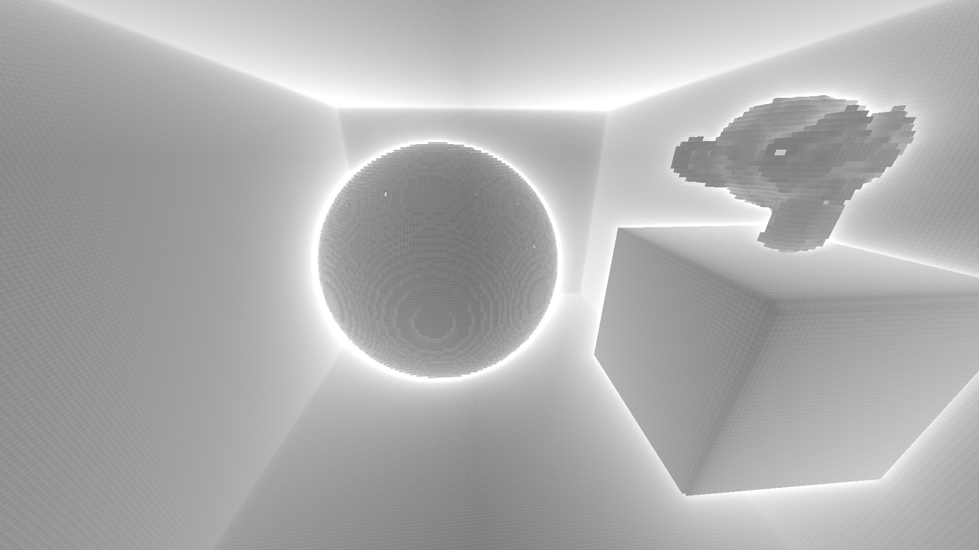
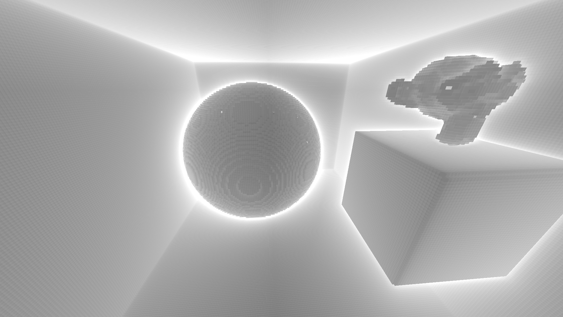
The voxelization produces three volumes: the albedo map, the normal map, and (after SDF computation) the SDF map.
Box scene:
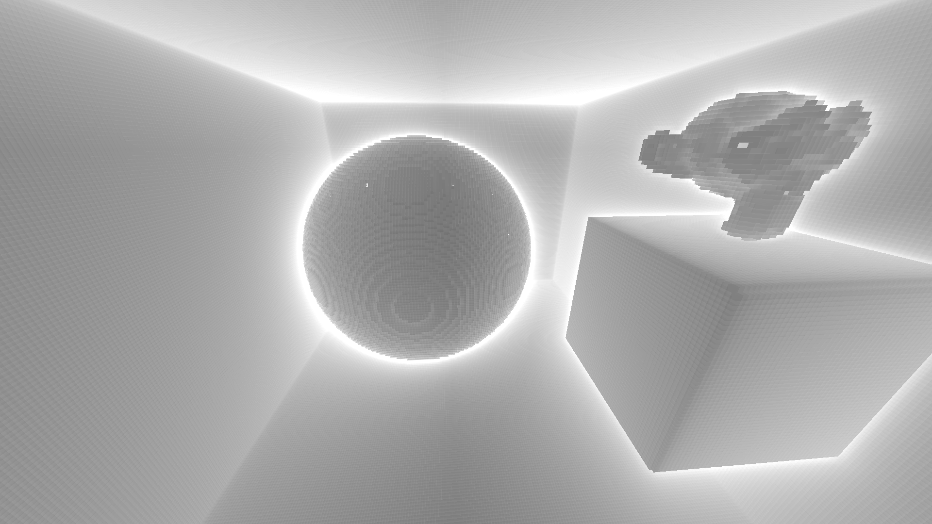
Sponza scene:
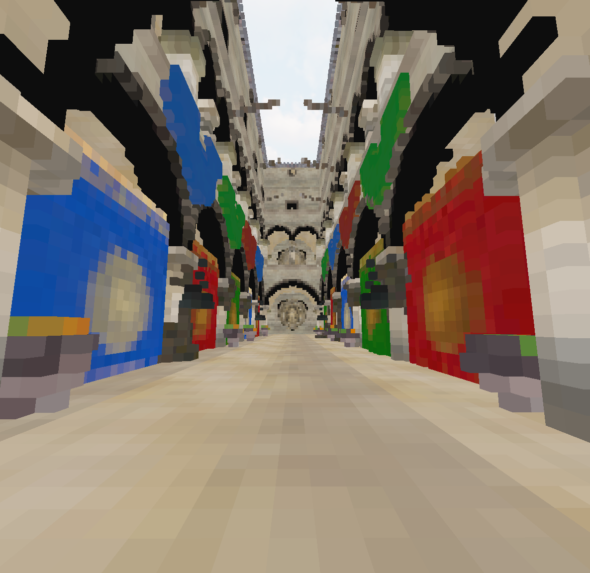
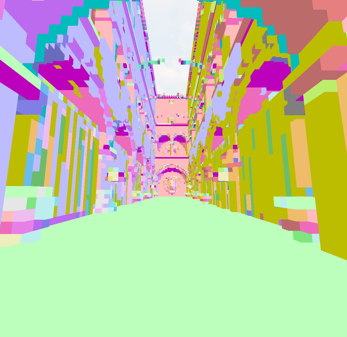
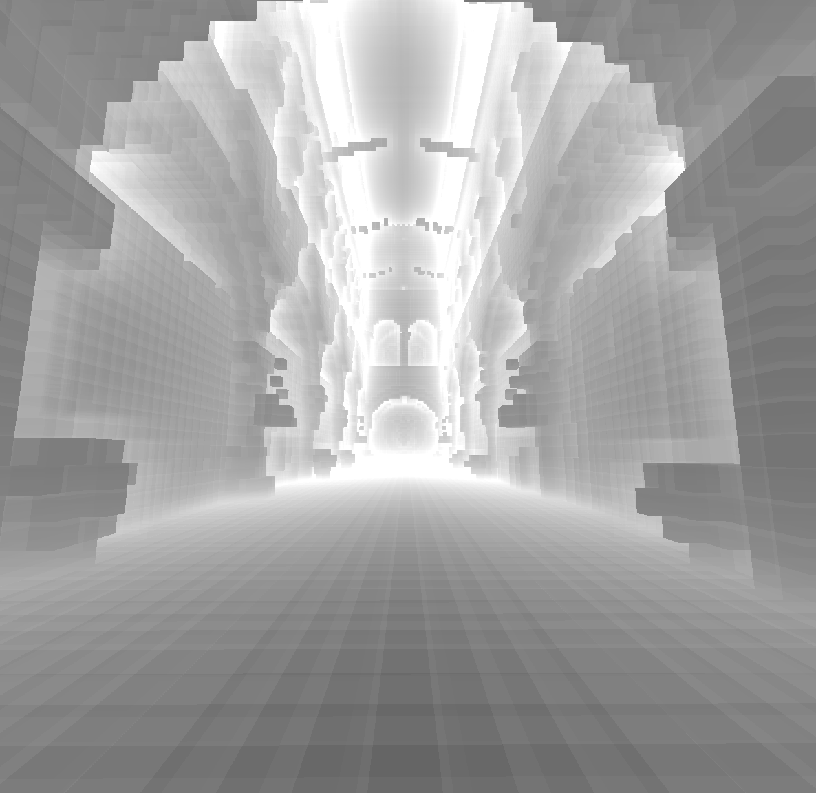
Albedo (left), normal direction encoded as color (center), and SDF distance field (right, brighter = farther from geometry).
Normal Encoding Strategies
Surface normals must be stored in the alpha channel of the R8G8B8A8_UNORM albedo volume. A zero alpha value serves as the voxel presence bit: a voxel is solid if and only if . The remaining 255 non-zero values encode the surface normal direction. Three strategies were evaluated.
6-Direction (Face-Aligned)
The normal is quantized to the nearest axis-aligned face direction, yielding six possible values:
Encoding and decoding require no arithmetic beyond an index lookup. The quantization error is large for oblique normals.
26-Direction (Face, Edge, and Corner)
The normal is quantized to the nearest vertex of the integer lattice with the origin excluded, giving 26 candidate directions. Each is subsequently normalized:
This scheme provides better angular coverage than 6-direction at no additional decode cost, but still produces visible faceting on curved surfaces.
Octahedral Encoding
Octahedral encoding establishes a bijective mapping between and the unit square, distributing all 255 available levels uniformly over the sphere. The scheme projects a unit normal onto the unit sphere:
For the lower hemisphere (), the projection is folded into the unit square:
The two components are then quantized to 4-bit unsigned integers and packed into a single byte:
This makes full use of all 255 levels and distributes quantization error uniformly over , at the cost of a small number of additional ALU instructions at decode time. Below is the GLSL implementation used in the project:
vec2 encodeOctahedral(vec3 n) {
    n = normalize(n);
    n /= (abs(n.x) + abs(n.y) + abs(n.z));
    vec2 oct = n.z >= 0.0 ? n.xy : (vec2(1.0) - abs(n.yx)) * sign(n.xy);
    return oct * 0.5 + 0.5;
}

float packNormal8(vec3 n) {
    vec2 oct = encodeOctahedral(n);
    uvec2 q = uvec2(clamp(oct, 0.0, 1.0) * 15.0 + 0.5);
    return float((q.x << 4) | q.y) / 255.0;
}

vec3 decodeOctahedral(vec2 oct) {
    oct = oct * 2.0 - 1.0;
    vec3 n = vec3(oct, 1.0 - abs(oct.x) - abs(oct.y));
    float t = max(-n.z, 0.0);
    n.xy += vec2(n.x >= 0.0 ? -t : t, n.y >= 0.0 ? -t : t);
    return normalize(n);
}

vec3 unpackNormal8(float pack) {
    uint bits = uint(pack * 255.0 + 0.5);
    vec2 q = vec2((bits >> 4) & 0xFu, bits & 0xFu) / 15.0;
    return decodeOctahedral(q);
}
Interactive Comparison
The following demo renders a sphere with normals encoded and decoded through each strategy. The color represents the decoded normal direction (RGB = XYZ mapped to [0,1]). The 6-direction mode shows extreme banding, 26-direction shows visible faceting, and octahedral produces a smooth gradient.
Bijective mapping from S² to the unit square. All 255 levels distributed uniformly over the sphere, minimal quantisation error.
Experimental Comparison
The following renders show the effect on diffuse GI (Box scene, curved geometry):
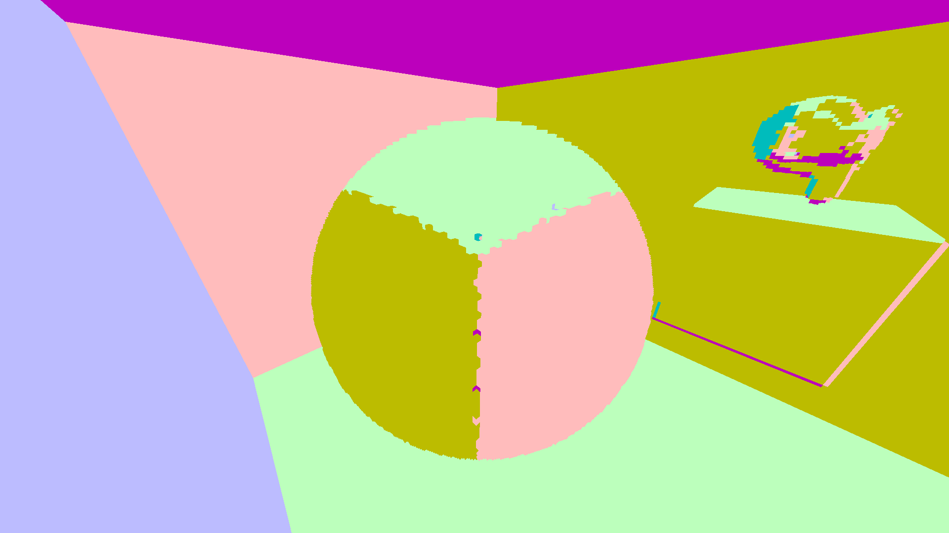
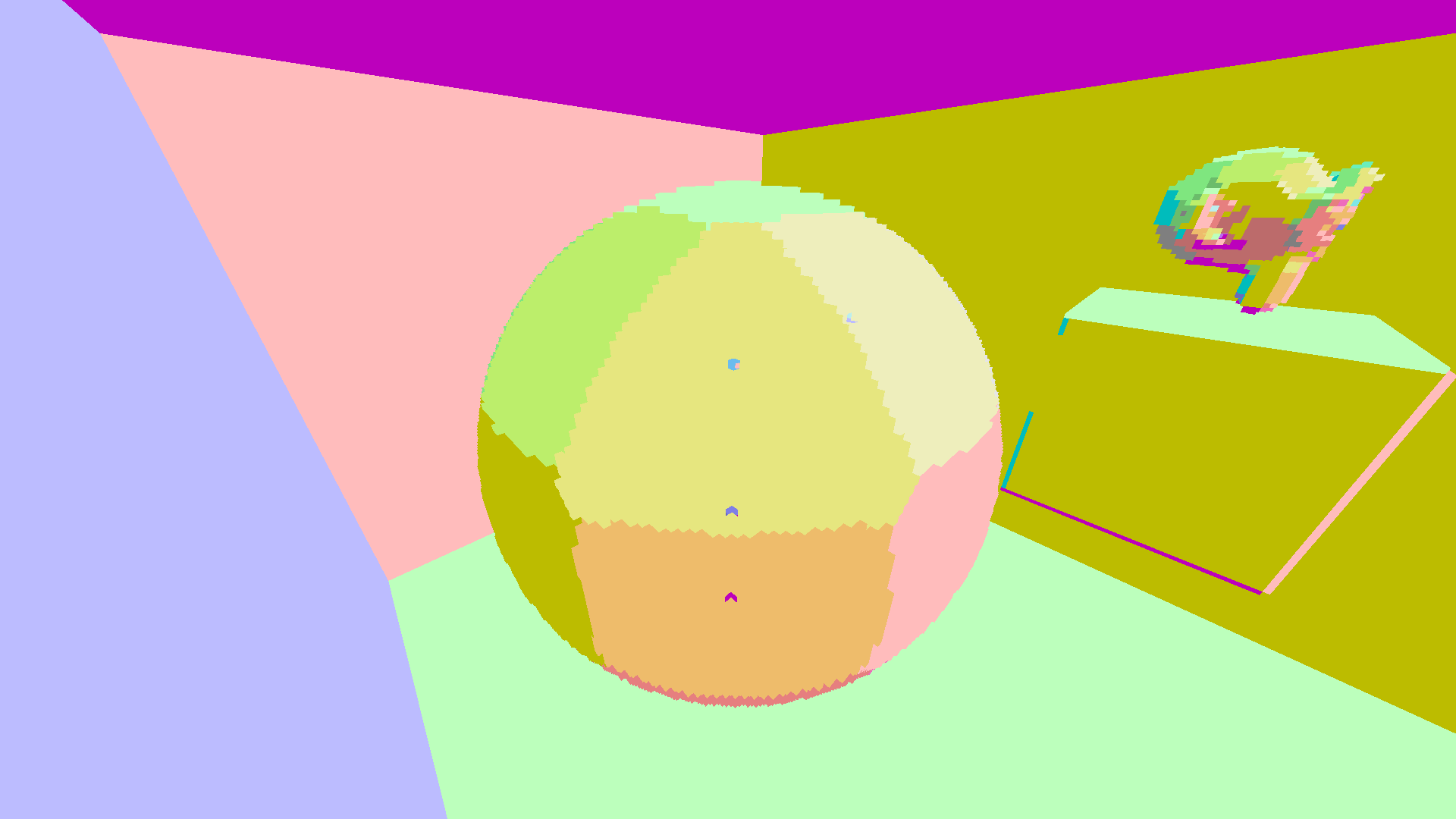
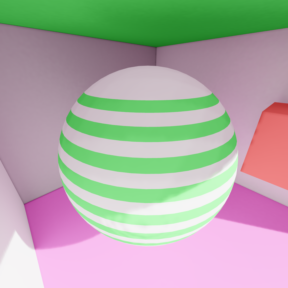
Diffuse GI with 6-direction normals (left), 26-direction (center), and octahedral (right). Note banding on the curved sphere with coarser encodings.
Experimental comparison confirmed that octahedral encoding provides meaningfully better results for surfaces with high normal variation. For flat geometry the difference is minimal, but octahedral is recommended as the default since the decode overhead is negligible. There is no additional cost during matrix construction since both encoding and decoding are GPU-side operations.
Signed Distance Field Computation
Visibility queries during form factor computation require traversing the voxel volume. Raw voxel traversal (DDA) is correct but slow for rays crossing large empty regions. To accelerate this, a signed distance field is precomputed from the voxel volume, enabling rays to skip empty space in large steps during raymarching.
Jump Flood Algorithm
The SDF is computed via the Jump Flood Algorithm (JFA), a standard parallel algorithm that produces a Voronoi diagram (and therefore a distance field) on the GPU. JFA runs in a series of double-buffered passes over the volume; the number of passes is:
In pass (counting from ), every voxel examines its neighbors at offset in each cardinal direction. If a neighbor holds a seed (solid voxel position) closer than the current best, the current voxel adopts that seed. After all passes, each voxel knows its nearest solid voxel and thus its unsigned distance to the nearest surface.
The key property is that JFA converges to the correct Voronoi diagram in logarithmic passes rather than the linear passes required by a naive flood fill. The resulting SDF is an approximation (not necessarily tight), but serves as a valid lower bound on the distance to the nearest occupied voxel along any ray, which is sufficient to preserve raymarching correctness at the cost of reduced skipping efficiency on strongly non-cubic AABBs.
Interactive JFA Demo
The following demo implements JFA on a 2D grid. Click to place seeds, then step through the algorithm to observe how the distance field propagates in logarithmic passes. Each cell is colored by its distance to the nearest seed.
Jump Flood Algorithm on a 64x64 grid. Each cell is colored by its nearest seed (Voronoi regions), with brightness modulated by distance (closer = brighter). White borders show the Voronoi cell boundaries. Click on the grid to place new seeds. The algorithm converges in log₂(N) passes.
Reference Implementation
The core evaluation logic of JFA in the 2D reference plotter:
evaluate(seed, neighbor, k) {
    if (neighbor[0] >= this.N || neighbor[0] < 0) return;
    if (neighbor[1] >= this.N || neighbor[1] < 0) return;

    var p = this.values[seed[0]][seed[1]];
    var q = this.values[neighbor[0]][neighbor[1]];

    if (p == null && q != null) {
        this.values[seed[0]][seed[1]] = this.values[neighbor[0]][neighbor[1]];
        this.values[seed[0]][seed[1]].distance = this.evaluateDistance(seed);
        return;
    }
    if (p != null && q != null) {
        var dq = this.evaluateDistance(neighbor);
        var dp = this.evaluateDistance(seed);
        if (dq < dp) {
            this.values[seed[0]][seed[1]] = this.values[neighbor[0]][neighbor[1]];
            this.values[seed[0]][seed[1]].distance = dq;
        }
    }
}

iterate() {
    for (var i = 0; i < this.N; i++) {
        for (var j = 0; j < this.N; j++) {
            var seed = [i, j];
            this.evaluate(seed, [i,     j + this.k], this.k);
            this.evaluate(seed, [i - this.k, j    ], this.k);
            this.evaluate(seed, [i + this.k, j    ], this.k);
            this.evaluate(seed, [i,     j - this.k], this.k);
        }
    }
    this.k = this.k / 2;
}
The final SDF volume is a single-channel 3D texture used exclusively to accelerate ray marching during form factor construction.
Solid Voxel List
Before constructing the form factor matrix, all solid voxels are compacted into a linear buffer called the SolidVoxelList. This serves two purposes:
- Matrix construction iterates only over solid voxels, skipping empty space entirely.
- The buffer establishes a stable mapping between entries of the radiance vector (indexed during Jacobi iteration) and voxel positions in the 3D radiance texture (indexed during scatter and forward shading).
The buffer layout (std430 alignment):
- Header (16 bytes): atomic counter for total solid voxel count.
- Entry (32 bytes each): voxel coordinates as
uint, encoded normal asuint, albedo asvec3, padding.
A compute shader iterates over every voxel in the volume, tests the alpha-channel presence bit, and atomically appends solid voxels to the list. A companion ReverseMap (a 3D texture with R32_UINT format) is simultaneously populated, mapping each integer voxel position back to its index in the SolidVoxelList. This inverse map is used in the scatter pass to write radiance at the correct list position.
The solid voxel counts for the test scenes at are:
| Scene | Triangles | Solid Voxels () |
|---|---|---|
| AbstractPark | 3 820 | 693 691 |
| Arena | 5 187 | 45 290 |
| Box | 5 022 | 450 793 |
| Sponza | 262 267 | 441 511 |
Form Factor Matrix Construction
The transport matrix is constructed stochastically on the GPU. For each solid voxel , the shader fires cosine-weighted rays sampled from a jittered Hammersley sequence over the hemisphere defined by voxel 's surface normal.
Hammersley Low-Discrepancy Sampling
The Hammersley sequence is a low-discrepancy point set constructed by pairing the Van der Corput radical-inverse function in base 2 with uniform stratification over samples. For hemisphere ray generation, each pair is mapped to a cosine-weighted direction via:
This provides superior hemisphere coverage compared to pseudo-random sampling, which is important since the matrix construction budget is fixed at rays per voxel.
Weight Computation and Storage
Each ray that hits a visible solid voxel (with incidence ) contributes an entry to row of the sparse matrix with weight:
This is the unbiased Monte Carlo estimate of the geometric form factor under cosine-weighted sampling. Visibility is evaluated by either DDA traversal on the integer voxel grid or SDF raymarching (see below).
The matrix is stored in a fixed-size CSR-like format: a flat buffer of (column-index, weight) pairs for each row, with a maximum of entries per row. The fixed-size layout avoids dynamic allocation on the GPU at the cost of wasted memory for voxels with fewer than visible neighbors.
DDA vs. SDF Raymarching
Two traversal strategies are available for the ray-voxel intersection during matrix construction:
DDA (Amanatides-Woo voxel traversal): Steps through the voxel grid one face at a time. Guaranteed to intersect every solid voxel the ray passes through. Reference-correct but traverses every empty voxel individually.
SDF raymarching: Uses the precomputed distance field to skip ahead by the minimum guaranteed distance to the nearest surface, approximately doubling traversal speed on sparse scenes. The SDF approximation from JFA is not tight, so the marcher may occasionally overshoot and miss a near-surface interaction. Experimentally, this produces slightly lower-intensity indirect shadows in edge cases, but no visible quality difference in typical scenes.
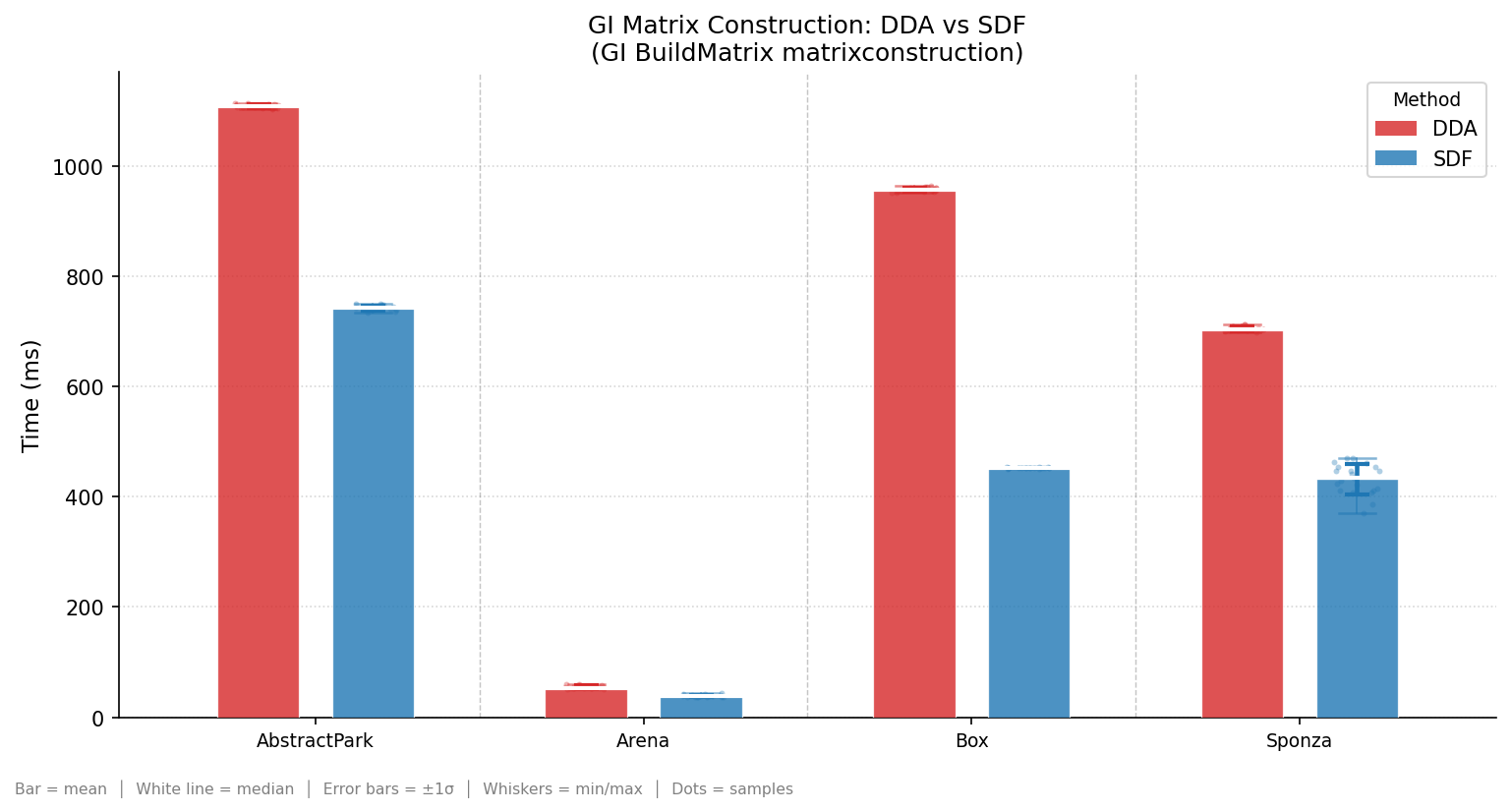
Matrix construction time across scenes. Blue: SDF raymarching. Red: DDA traversal. SDF is approximately 2× faster on average.
Relaxation Parameter
Multiple rays can land on the same destination voxel when source and destination are spatially close relative to voxel size. This produces duplicate column entries in a row, causing row weights to sum above 1.0, which violates energy conservation and prevents Jacobi convergence. Sorting rows and deduplicating would be expensive on the GPU. Instead, a relaxation parameter scales the total propagation:
Experimental results across all four test scenes showed optimal visual agreement with Cycles reference renders for . The parameter is scene-dependent and tunable at runtime.
Low-Probability High-Energy Paths
A known limitation of the stochastic sampling approach: rays that hit a very small but extremely energetic region may be missed if the row budget is exhausted before they are sampled. Because neighboring voxels may have different row entries, this can produce localized noise from matrix discontinuities. Increasing reduces this noise at linear cost to both memory and construction time.
Per-Frame Pipeline
Light Gathering
A compute kernel iterates over every solid voxel in the SolidVoxelList and gathers current direct lighting into an EmissionBuffer. The computation is identical to a standard forward shader for the supported light types:
- Spotlights / Sunlights: Shadow map visibility test per voxel, using the same PCF shadow map generated for the forward pass.
- Emissive geometry: Read directly from the emissive channel of the albedo volume, populated during voxelization.
- Omnilights: Cubemap shadow mapping (not implemented in this version due to time constraints).
This pass is the most extensible part of the algorithm. Any direct lighting source that can be evaluated at a 3D world position can be incorporated into the emission buffer without modifying any other pipeline stage.
Radiosity Solver (Jacobi SpMV)
The core solver performs one step of Jacobi power iteration per frame:
where is the per-voxel radiance vector (one vec4 per solid voxel), is the current emission vector, and is the albedo-weighted form factor matrix. The relight converges to a steady state in several iterations, after which it can be cached until lighting changes.
Double buffering. Jacobi iteration reads the previous state while writing the next, requiring a ping-pong pair of radiance buffers. The GPU-equivalent of Gauss-Seidel (which updates in-place) would converge faster but requires reading and writing the same buffer with ordering guarantees, which is not efficiently achievable in a compute shader.
Workgroup SpMV. Each workgroup is responsible for computing a single dot product (one row of the matrix-vector product). The workgroup size is fixed to 64 threads, matching the RDNA3 wavefront width.
For a row of size , each thread is responsible for entries at indices within the row. Thread reads its assigned entries, accumulates partial results into shared memory, and then participates in a barrier-synchronized tree reduction:
- Each thread accumulates its partial sum into
sharedMem[localID]. - A sequence of barrier-synchronized reduction steps halves the active thread count each time.
- Thread 0 writes the final scalar result to the output radiance buffer at the correct solid-voxel index.
This pattern is efficient because all threads in a workgroup read contiguous ranges of the row, maintaining good cache locality on the SSBO.
Light Scattering
After the Jacobi iteration, the updated radiance lives in the flat SSBO RadianceBuffer. For efficient sampling in the forward shader, it must be written into a 3D texture (RadianceTexture, RGBA16F) indexed by voxel position. A compute shader dispatches one invocation per solid voxel and performs this scatter using the voxel coordinates stored in the SolidVoxelList.
The RadianceTexture is cleared at the start of each scatter pass to remove stale radiance from the previous iteration.
Shadow hard-edge correction. The RadianceBuffer contains embedded direct light gathered in the EmissionBuffer. If written directly to the RadianceTexture and sampled in the forward shader, direct light would be applied twice: once from the voxel volume sample and once from the forward shader's own direct lighting pass. To correct this, the scatter pass subtracts the emission before writing:
where is the value written to the texture, is the accumulated radiosity result, and is the direct emission. A side effect of skipping this subtraction is that direct light values remain embedded in the RadianceTexture, allowing them to appear in specular reflections computed by the raytracer in the forward pass. This creates a design trade-off between shadow boundary accuracy and reflection quality.
Pre-multiplied alpha sampling. When the forward shader samples the RadianceTexture using a fragment's world position, the sample may land on a neighboring empty voxel (black in the texture). Linear filtering with pre-multiplied alpha corrects this: the alpha channel stores a presence value (1.0 for solid, 0.0 for empty), and the sampled color is divided by the interpolated alpha:
An additional blur kernel over the 3D sample further smooths radiance and suppresses noise from low-probability high-energy paths. Since radiosity radiance has inherently low spatial frequency, this introduces minimal error while meaningfully reducing visible artifacts.
Specular Extensions
Specular Light Tracing
Since the voxelization stage produces all data necessary for DDA ray traversal, a voxel-space ray tracer in the forward shader can evaluate specular indirect paths at shading time.
For each fragment, rays are stochastically generated within the specular cone defined by the fragment's surface normal, jittered by an amount proportional to the PBR roughness parameter (wider cone = rougher surface). Each ray is traced using DDA through the voxel volume until it hits a solid voxel or escapes the volume. The radiance at the hit voxel is read from the RadianceTexture. Results from all rays are averaged and weighted by PBR coefficients (Cook-Torrance BRDF with GGX NDF) to produce the specular indirect contribution.
The final GI value per fragment is the sum of:
- Diffuse indirect: sampled directly from the RadianceTexture at the fragment's world position.
- Specular indirect: averaged over stochastically traced rays in the specular cone.
A practical note: this approach can produce significant specular aliasing for surfaces with high-frequency normal variation. Using geometric normals instead of interpolated normals for the specular cone direction reduces this, at the cost of some shading smoothness.
SD* — Specular Writeback
As a novel contribution, the specular value computed during forward shading can be written back into the emission volume via imageStore, allowing specular contributions to re-enter the radiosity solver in subsequent iterations. This creates a specular-to-diffuse (SD*) transport path without requiring per-frame ray traversal in the GI solver itself.
The primary challenge is memory contention: many fragment shader threads may attempt to write to the same voxel simultaneously. A proximity mask limits writes to at most one representative fragment per voxel cell.
Let be the fragment world position, the camera position, and the surface normal.
Step 1 — Camera distance weighting. A sub-linear distance factor:
softens the falloff with camera distance.
Step 2 — Voxel-space projection. The fragment is projected into voxel space , and its fractional cell position gives its position within the voxel cell.
Step 3 — Normal-weighted centering. Each axis of is blended toward the voxel center (0.5) proportionally to the surface normal alignment with that axis:
A face perpendicular to axis () collapses all its fragments to the same voxel-center coordinate along that axis.
Step 4 — Proximity score. Distance from the blended grid point to the voxel center:
Normalized by camera distance and clamped:
Step 5 — Mask condition. A fragment issues the imageStore only if for threshold . This heuristically selects at most one representative fragment per voxel cell under normal viewing conditions.
Experimentally, SD* adds perceptual realism through IBL-like indirect specular contributions but introduces significant temporal flickering and carries a performance cost several times higher than regular shading. A more robust implementation would write specular data to a color attachment and process writes in a dedicated compute pass, avoiding fragment shader contention entirely. This remains as future work.
Memory Analysis
Let be the total voxel count, the number of solid voxels, the GPU solid-list capacity rounded up to the next power of two (for lock-free atomic allocation), and the per-row form-factor budget.
Volume buffers (seven 3D textures over the full grid):
Three textures at 8 B/voxel (R16G16B16A16_SFLOAT): radiance ping, radiance pong, JFA work volume. Three at 4 B/voxel (R8G8B8A8_UNORM or R32_UINT): albedo, JFA seed scratch, ReverseMap:
Matrix GI buffers (allocated against ):
The solid list stores 8 uint32 fields per entry (32 B) plus a 16 B header; each form-factor entry stores a column index and quantized weight (2 uint32 = 8 B); row counters use 4 B; and three vec4 arrays of 16 B each hold the Jacobi solution ping-pong pair and the emission cache:
The dominant term is (the matrixHits buffer), accounting for approximately 97% of at the default parameters ().
Total:
Both terms scale as , but carries the coefficient , making it the dominant cost in practice. For the Sponza scene at (, , , ):
| Subsystem | Buffer | Format | Size (MB) |
|---|---|---|---|
| Voxel Volumes | voxelAlbedo | RGBA8_UNORM | 16.41 |
voxelRadiance ping | RGBA16F | 32.83 | |
voxelRadiance pong | RGBA16F | 32.83 | |
jfaScratch | R32_UINT | 16.41 | |
jfaWork | RGBA16F | 32.83 | |
reverseMap | R32_UINT | 16.41 | |
| Volume subtotal | 147.72 | ||
| Matrix GI | solidList | uint32[] | 32.00 |
matrixHits | uint32[] | 3 072.00 | |
rowCounts | uint32[] | 4.00 | |
radianceXBuf | vec4[] | 16.00 | |
emissionBuf | vec4[] | 16.00 | |
| Matrix subtotal | 3 140.00 | ||
| Grand total | 3 287.72 |
The matrixHits buffer alone accounts for 93% of total GPU memory consumption at these parameters. Matrix compression (e.g., block SVD, hierarchization) is the most impactful direction for reducing this footprint.
Experimentation
Test Platform
| Component | Detail | Specification |
|---|---|---|
| CPU | Model | AMD Ryzen 9 7900 |
| Cores | 12C / 24T @ 4.34 GHz | |
| GPU | Model | AMD Radeon RX 7700 XT |
| VRAM | 12 GB GDDR6 | |
| Subgroup | 64 lanes (RDNA3) | |
| API | Vulkan | 1.4.348 |
| Driver | RADV Mesa 26.1.1 | |
| OS | Arch Linux |
Default experimental parameters:
| Parameter | Default |
|---|---|
| Voxel map resolution | |
| Matrix row size | 384 |
| Normal encoding | Octahedral |
| Build matrix mode | DDA |
| Edge removal | Disabled |
| Sample blurred radiance | Enabled |
| Pre-multiplied alpha | Enabled |
| Specular writeback | Disabled |
| Specular ray count | 2 per fragment |
| Diffuse ray count | 384 per voxel |
| Viewport |
Voxel Resolution
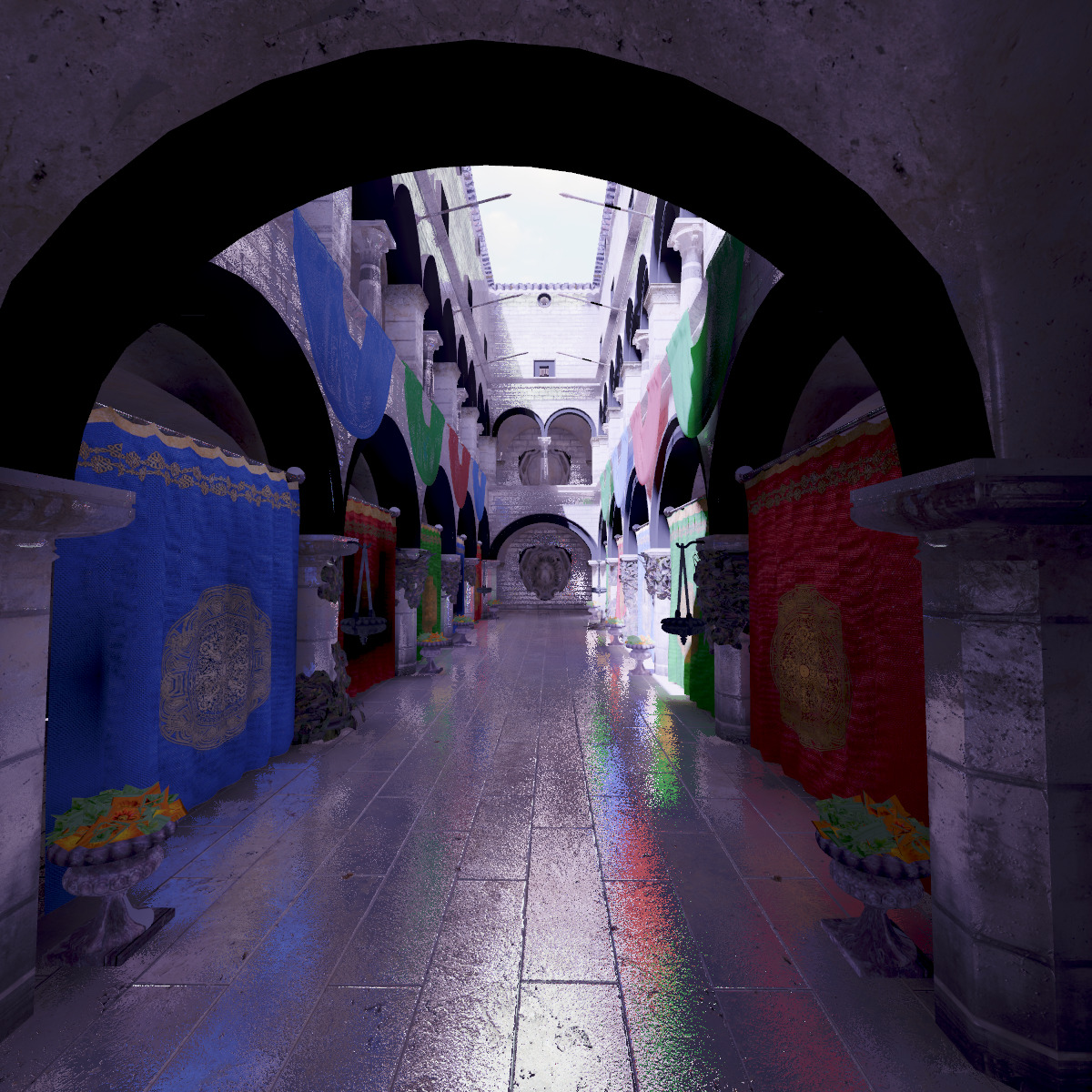
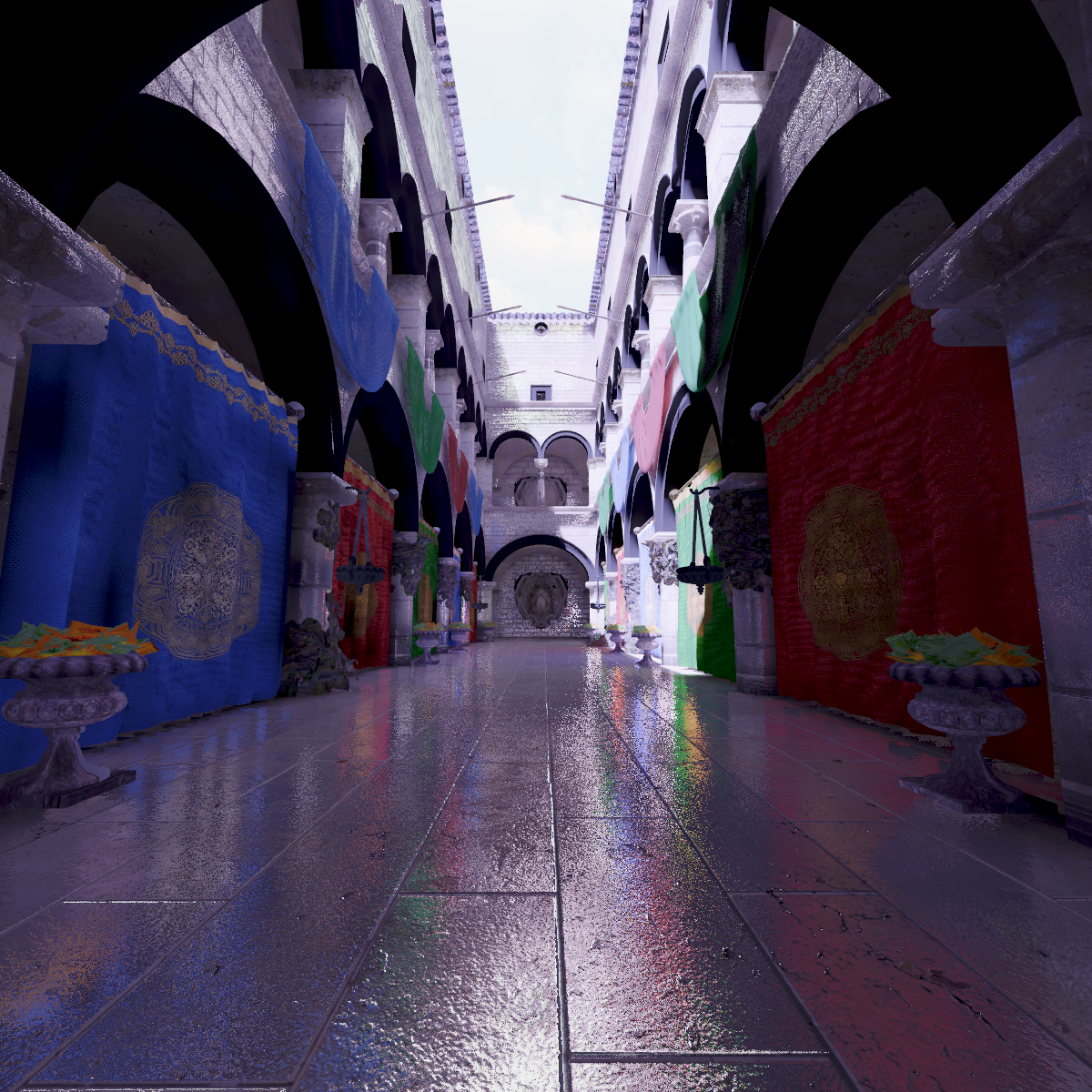
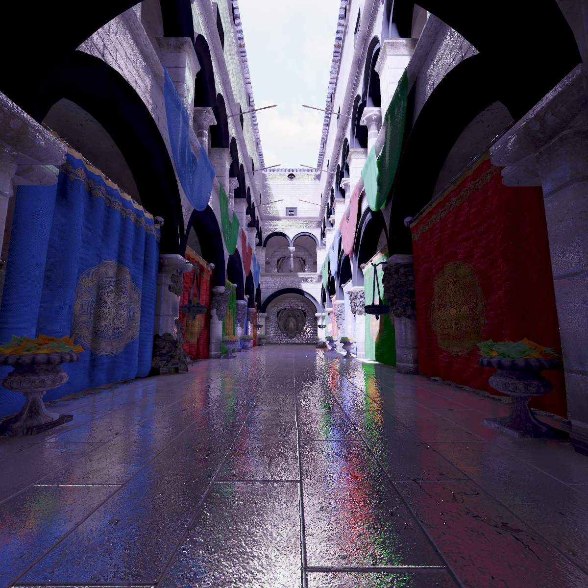
(left), (center), (right). Computation time scales cubically with . Lower resolutions produce smoother results with fewer artifacts from high-frequency normals, at the cost of spatial detail and light-leak through thin geometry.
At , the Sponza voxel edge length is approximately 29 cm — coarser than the scene's thinnest geometry, which allows some light leaking. At (14.5 cm), the main visible artifacts are reduced. At , diminishing returns are observed in quality while construction time grows significantly.
Relaxation Parameter
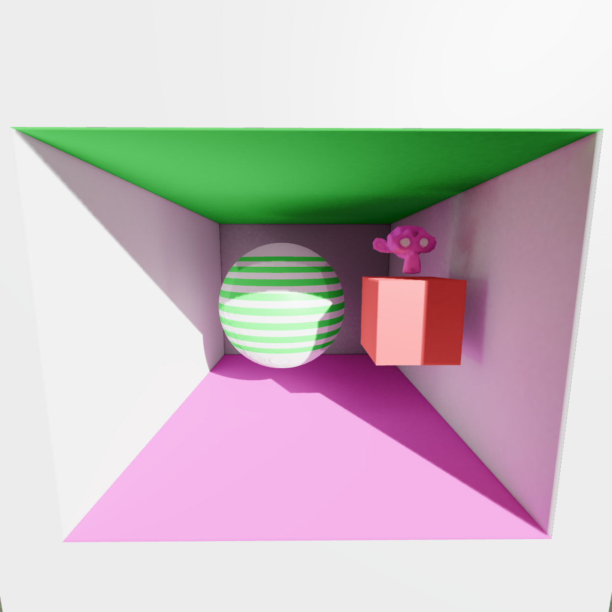
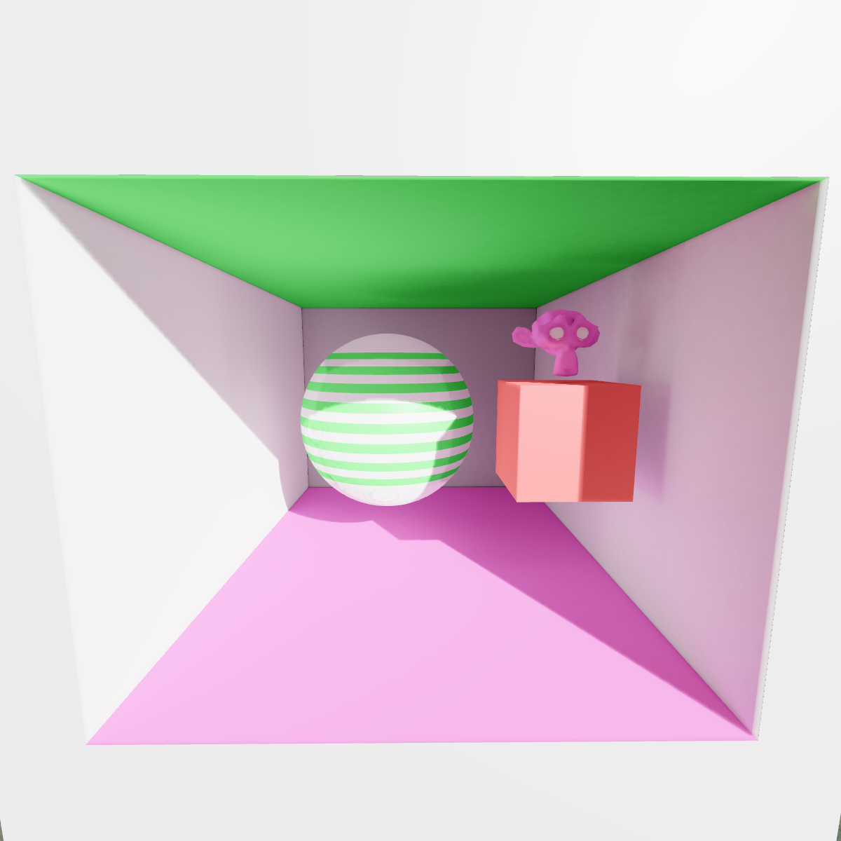
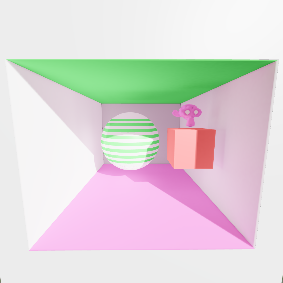
(left), (center), (right). The optimal range matches Cycles reference renders most closely. Values approaching 1.0 may fail to converge if row weights sum above 1 due to duplicate entries.
DDA vs. SDF Matrix Construction
Across all four test scenes, SDF raymarching reduces matrix construction time by approximately 2× compared to DDA, with no perceptible difference in final GI quality for typical lighting configurations. In edge cases with tightly-spaced geometry, SDF can miss near-surface interactions due to the approximate JFA distance field, producing slightly lower-intensity indirect shadows.
Normal Encoding
The 6- and 26-direction schemes require no arithmetic at decode time and trivially preserve the presence bit. The octahedral scheme makes full use of all 255 levels and distributes quantization error uniformly over at the cost of a small number of additional ALU instructions. For surfaces with significant normal variation (curved geometry), octahedral encoding is visibly superior. For flat planar geometry, the difference is negligible. Octahedral encoding is recommended as the default.
Relight Performance
One Jacobi iteration (the entire relight step) runs in 2–4 ms on the AMD RX 7700 XT. The bottleneck is memory bandwidth rather than compute: each iteration reads the full matrixHits buffer (3 GiB at default parameters) to perform one SpMV pass. Performance scales directly with memory bandwidth. The AMD 7700 XT is particularly strong in this regard; performance on bandwidth-limited mobile or integrated GPUs would be substantially worse.
Comparison Against Reference
The diffuse indirect component was compared against Cycles (path-traced ground truth) and EEVEE (real-time) for the same lighting configuration. The main visible difference against Cycles is shadow boundary quality (PCF shadow maps vs. soft ray-traced shadows), not the GI computation itself. The indirect color bleeding and overall energy distribution match Cycles closely for all four test scenes.
Limitations
GPU memory. The view factor matrix dominates memory consumption. At with , the Sponza scene requires over 3 GiB of VRAM for the GI subsystem alone. Scaling to or larger scenes rapidly exceeds available VRAM on consumer hardware.
Static geometry only. The form factor matrix encodes visibility between all patch pairs at construction time. Any change in scene geometry (moving an object, opening a door) invalidates the matrix and requires reconstruction. Partial matrix updates for small changes are theoretically possible but not implemented.
Memory bandwidth bottleneck. The per-frame relight reads the entire matrix per iteration. At 3 GiB and 2–4 ms, this saturates the memory bus at ~750 GB/s, which is close to the theoretical peak bandwidth of the RX 7700 XT. Performance on bandwidth-limited hardware degrades proportionally.
Specular writeback (SD).* The proximity mask strategy reduces contention but does not eliminate it. The result suffers from temporal flickering due to frame-to-frame variation in which fragments are selected. The correct solution (writing to a color attachment and processing in compute) was not implemented within the scope of this project.
Specular aliasing. The voxel-space DDA ray tracer in the forward shader produces aliasing for high-frequency normal variation. Using geometric normals for the ray direction mitigates this at the cost of shading accuracy.
Conclusions and Future Work
The experimental results support the central hypothesis: a precomputed sparse radiosity matrix enables competitive real-time global illumination with a per-frame cost of 2–4 ms on current hardware, without per-frame ray traversal. The diffuse indirect component closely matches path-traced references. The specular extension, while approximate, adds perceptual realism at low additional cost.
The primary constraint is GPU memory. At practical resolutions, the transport matrix requires several gigabytes of VRAM, which limits scalability to scenes that fit within the memory budget of high-end consumer hardware.
Future directions:
- Matrix compression: randomized block SVD, hierarchical radiosity, or grouped-patch compression to reduce the dominant memory term while preserving transport accuracy.
- Variable-resolution patches: sparse voxel representations with non-uniform in-world patch sizes, allowing high-detail regions near the camera and coarser patches farther away.
- Dynamic partial updates: selective matrix recomputation for moving geometry, reusing unchanged rows and reconstructing only affected regions.
- Async compute overlap: the relight pass is memory-bound while the forward pass is compute-bound; scheduling them in parallel on separate GPU engines could improve overall frame time.
- SD via compute*: replacing the fragment-shader writeback with a color attachment and a dedicated compute pass would eliminate contention and enable robust specular-to-diffuse transport.
The most practical near-term application is as an optional offline-to-realtime GI backend for renderers such as EEVEE, bridging the quality gap with Cycles at a fraction of the render time (Cycles takes minutes per frame; Immediate Radiosity runs in under 4 ms after a one-time setup cost).
Novel Contributions
- SD* (Specular Writeback): a new transport path that writes specular contributions from the forward shader back into the diffuse radiance cache, enabling indirect specular propagation through subsequent radiosity iterations without per-frame ray traversal in the solver.
- Stochastic SDF raymarching for form factor computation: using the JFA-computed approximate SDF to accelerate matrix construction, achieving approximately 2× speedup over DDA with negligible quality loss.
- Comprehensive parameter study across four scenes: voxel resolution (), matrix row size (), normal encoding strategy (6-direction, 26-direction, octahedral), traversal mode (DDA vs. SDF), relaxation parameter (), sampling mode (pre-multiplied alpha, blur kernel).
- Full GPU-only implementation: all passes including voxelization, JFA, matrix construction, Jacobi iteration, and scatter are compute shaders with no CPU-side iteration. The only CPU involvement is dispatch call submission.
Technologies
- C++ / Vulkan / GLSL
- GPU compute shaders (SSBO-based SpMV, Jacobi power iteration)
- Signed distance fields via Jump Flood Algorithm
- Voxelization pipeline with geometry-shader dominant-axis projection
- Physically-based rendering (Cook-Torrance microfacet BRDF, GGX NDF, Disney parameterization)
- Low-discrepancy sampling (Hammersley / Van der Corput sequence)
- Sparse matrix storage (fixed-row CSR-like format)
- Pre-multiplied alpha volume sampling